Learn R for Psychology Research: A Crash Course
Introduction
I wrote this for psychologists who want to learn how to use R in their research right now. What does a psychologist need to know to use R to import, wrangle, plot, and model their data today? Here we go.
Foundations: People and their resources that inspired me.
- Dan Robinson [.html] convinced me that beginneRs should learn tidyverse first, not Base R. This tutorial uses tidyverse. All you need to know about the differnece is in his blog post. If you’ve learned some R before this, you might understand that difference as you go through this tutorial.
- If you want a more detailed introduction to R, start with R for Data Science (Wickham & Grolemund, 2017) [.html]. The chapters are short, easy to read, and filled with simple coding examples that demonstrate big principles. And it’s free.
- Hadley Wickham is a legend in the R community. He’s responsible for the tidyverse, including ggplot2. Read his books and papers (e.g., Wickham, 2014). Watch his talks (e.g., ReadCollegePDX, October 19, 2015). He’s profoundly changed how people think about structuring and visualizing data.
Need-to-Know Basics
Install R and R Studio (you need both in that order)
Understand all the panels in R Studio
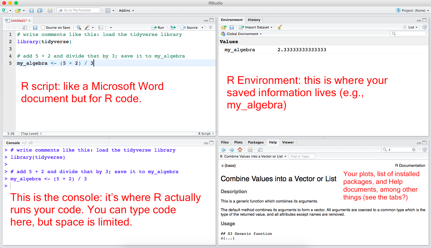
Four panels in R Studio
Packages: They’re like apps you download for R
“Packages are collections of R functions, data, and compiled code in a well-defined format. The directory where packages are stored is called the library. R comes with a standard set of packages. Others are available for download and installation. Once installed, they have to be loaded into the session to be used.” [.html]
# before you can load these libraries, you need to install them first (remove the # part first):
# install.packages("tidyverse")
# install.packages("haven")
# install.packages("psych")
# install.packages("car")

library(tidyverse)
library(haven)
library(psych)
library(car)
Objects: They save stuff for you
“
object <- fuction(x), which means ‘object is created from function(x)’. An object is anything created in R. It could be a variable, a collection of variables, a statistical model, etc. Objects can be single values (such as the mean of a set of scores) or collections of information; for example, when you run an analysis, you create an object that contains the output of that analysis, which means that this object contains many different values and variables. Functions are the things that you do in R to create your objects.”
Field, A., Miles., J., & Field, Z. (2012). Discovering statistics using R. London: SAGE Publications. [.html]
c() Function: Combine things like thing1, thing2, thing3, …
“c” stands for combine. Use this to combine values into a vector. “A vector is a sequence of data ‘elements’ of the same basic type.” [.html] Below, we create an object called five_numbers. We are naming it for what it is, but we could name it whatever we want: some_numbers, maple_tree, platypus. It doesn’t matter. We’ll use this in the examples in later chunks of code.
# read: combine 1, 2, 3, 4, 5 and "save to", <-, five_numbers
five_numbers <- c(1, 2, 3, 4, 5)

# print five_numbers by just excecuting/running the name of the object
five_numbers
## [1] 1 2 3 4 5R Help: help() and ?
“The help() function and ? help operator in R provide access to the documentation pages for R functions, data sets, and other objects, both for packages in the standard R distribution and for contributed packages. To access documentation for the standard lm (linear model) function, for example, enter the command help(lm) or help(”lm“), or ?lm or ?”lm" (i.e., the quotes are optional)." [.html]
Piping, %>%: Write code kinda like you write sentences
The
%>%operator allows you to “pipe” a value forward into an expression or function; something along the lines of x%>%f, rather than f(x). See the magrittr page [.html] for more details, but check out these examples below.
Compute z-scores for those five numbers, called five_numbers
- see help(scale) for details
five_numbers %>% scale()## [,1]
## [1,] -1.2649111
## [2,] -0.6324555
## [3,] 0.0000000
## [4,] 0.6324555
## [5,] 1.2649111
## attr(,"scaled:center")
## [1] 3
## attr(,"scaled:scale")
## [1] 1.581139Compute Z-scores for five_numbers and then convert the result into only numbers
- see help(as.numeric) for details
five_numbers %>% scale() %>% as.numeric()## [1] -1.2649111 -0.6324555 0.0000000 0.6324555 1.2649111Compute z-scores for five_numbers and then convert the result into only numbers and then compute the mean
- see help(mean) for details
five_numbers %>% scale() %>% as.numeric() %>% mean()## [1] 0Tangent: most R introductions will teach you to code the example above like this:
mean(as.numeric(scale(five_numbers)))## [1] 0
- I think this code is counterintuitive. You’re reading the current sentence from left to right. That’s how I think code should read like: how you read sentences. Forget this “read from the inside out” way of coding for now. You can learn the “read R code inside out” way when you have time and feel motivated to learn harder things. I’m assuming you don’t right now.
Functions: they do things for you
“A function is a piece of code written to carry out a specified task; it can or can not accept arguments or parameters and it can or can not return one or more values.” Functions do things for you. [.html]
Compute the num of five_numbers
- see help(sum) for details
five_numbers %>% sum()## [1] 15Compute the length of five_numbers
- see help(length) for details
five_numbers %>% length()## [1] 5Compute the sum of five_numbers and divide by the length of five_numbers
- see help(Arithmetic) for details
five_numbers %>% sum() / five_numbers %>% length()## [1] 3Define a new function called compute_mean
compute_mean <- function(some_numbers) {
  some_numbers %>% sum() / some_numbers %>% length()
}
Compute the mean of five_numbers
five_numbers %>% compute_mean()## [1] 3Tangent: Functions make assumptions; know what they are
What is the mean of 5 numbers and a unknown number, NA?
- see help(NA) for details
c(1, 2, 3, 4, 5, NA) %>% mean()## [1] NAIs this what you expected? Turns out, this isn’t a quirky feature of R. R was designed by statisticians and mathematicians.
NArepresents a value that is unknown. Ask yourself, what is the sum of an unknown value and 17? If you don’t know the value, then you don’t know the value of adding it to 17 either. Themean()function givesNAfor this reason: the mean of 5 values and an unknwon value isNA; it’s unknown; it’s not available; it’s missing. When you use functions in your own research, think about what the functions “assume” or “know”; ask, “What do I want the function to do? What do I expect it to do? Can the function do what I want with the information I gave it?”
Tell the mean() function to remove missing values
c(1, 2, 3, 4, 5, NA) %>% mean(na.rm = TRUE)## [1] 3Create data for psychology-like examples
This is the hardest section of the tutorial. Keep this is mind: we’re making variables that you might see in a simple psychology dataset, and then we’re going to combine them into a dataset. Don’t worry about specifcs too much. If you want to understand how a function works, use ?name_of_function or help(name_of_function).
Subject numbers
- read like this: generate a sequence of values from 1 to 100 by 1
- see help(seq) for details
subj_num <- seq(from = 1, to = 100, by = 1)

# print subj_num by just excecuting/running the name of the object
subj_num
## [1] 1 2 3 4 5 6 7 8 9 10 11 12 13 14 15 16 17
## [18] 18 19 20 21 22 23 24 25 26 27 28 29 30 31 32 33 34
## [35] 35 36 37 38 39 40 41 42 43 44 45 46 47 48 49 50 51
## [52] 52 53 54 55 56 57 58 59 60 61 62 63 64 65 66 67 68
## [69] 69 70 71 72 73 74 75 76 77 78 79 80 81 82 83 84 85
## [86] 86 87 88 89 90 91 92 93 94 95 96 97 98 99 100See those numbers on the left hand side of the output above? Those help you keep track of a sequence (i.e., line) of elements as the output moves to each new line. This is obvious in the example above because numbers correspond exactly to their position. But if these were letters or random numbers, that index or position (e.g., [14] “N”) tells you the position of that element in the line.
Condition assignments
- read like this: replicate each element of c(“control”, “manipulation”) 50 times, and then turn the result into a factor
- side: in R, factors are nominal variables (i.e., integers) with value labels (i.e., names for each integer).
- see help(rep) and help(factor) for details
condition <- c("control", "manipulation") %>% rep(each = 50) %>% factor()

# print condition by just excecuting/running the name of the object
condition
## [1] control control control control control
## [6] control control control control control
## [11] control control control control control
## [16] control control control control control
## [21] control control control control control
## [26] control control control control control
## [31] control control control control control
## [36] control control control control control
## [41] control control control control control
## [46] control control control control control
## [51] manipulation manipulation manipulation manipulation manipulation
## [56] manipulation manipulation manipulation manipulation manipulation
## [61] manipulation manipulation manipulation manipulation manipulation
## [66] manipulation manipulation manipulation manipulation manipulation
## [71] manipulation manipulation manipulation manipulation manipulation
## [76] manipulation manipulation manipulation manipulation manipulation
## [81] manipulation manipulation manipulation manipulation manipulation
## [86] manipulation manipulation manipulation manipulation manipulation
## [91] manipulation manipulation manipulation manipulation manipulation
## [96] manipulation manipulation manipulation manipulation manipulation
## Levels: control manipulationDependent Measure
Save 5 values that represent the sample sizes and the true means and standard deviations of our pretend conditions
sample_size <- 50
control_mean <- 2.5
control_sd <- 1
manip_mean <- 5.5
manip_sd <- 1
Introduce a neat function in R: rnorm()
rnorm stands for random normal. Tell it sample size, true mean, and the true sd, and it’ll draw from that normal population at random and spit out numbers. * see help(rnorm) for details
# for example
rnorm(n = 10, mean = 0, sd = 1)
## [1] 0.49894471 -0.32804955 0.50537413 -0.11556736 -0.08508432
## [6] 0.08209753 -0.19807435 -0.67604751 -1.40819698 0.65839239Randomly sample from our populations we made up above
control_values <- rnorm(n = sample_size, mean = control_mean, sd = control_sd)

manipulation_values <- rnorm(n = sample_size, mean = manip_mean, sd = manip_sd)
Combine those and save as our dependent variable
dep_var <- c(control_values, manipulation_values)

# print dep_var by just excecuting/running the name of the object
dep_var
## [1] 3.80435908 1.98433834 3.58911265 2.25427353 2.26939479
## [6] 3.00571297 1.79599758 3.78066987 2.57893735 0.41113928
## [11] 1.45297236 -0.26800475 0.94876854 2.72645231 2.11293954
## [16] 0.93341662 2.32122047 2.13377155 2.47441804 4.10472885
## [21] 2.87566838 1.61589446 1.40305547 1.17898161 3.45501450
## [26] 1.63901146 3.27007143 2.88237529 -0.01839347 1.34987475
## [31] 2.81149228 2.43357785 2.00504670 0.92384205 2.12499045
## [36] 2.81331542 4.16386024 3.37649612 3.00652454 3.56641968
## [41] 2.79969451 1.69841398 3.34037340 1.58360830 3.27350578
## [46] 2.21078116 2.28055121 1.24831449 4.25549097 2.28968369
## [51] 5.53075605 5.88079557 3.98853615 5.40940592 5.67097034
## [56] 6.57733121 4.95465727 4.74030459 7.07676495 5.84818695
## [61] 5.58482038 6.63561264 4.22953125 5.26021676 4.18271199
## [66] 6.28222681 5.09162940 4.15811312 4.22998668 6.46896233
## [71] 6.39382167 4.30209211 5.17371080 6.37887623 6.65385566
## [76] 4.99211078 5.80340366 6.05295369 4.41951254 4.76894952
## [81] 5.97968673 5.18637234 6.27683921 4.14482297 4.88000977
## [86] 3.52223543 5.10475171 5.12186433 3.99062501 5.86301456
## [91] 6.55805845 5.03726371 5.37350470 5.01889901 7.13802500
## [96] 5.18802629 6.02507734 6.59428100 5.23363327 4.44856252Create a potentially confounding variable or a control variable
in the code below, we multiply every value in dep_var by 0.5 and then we “add noise”: 100 random normal values whose true population has a mean = 0 and sd = 1. Every value in dep_var * 0.5 gets a random value added to it.
confound <- dep_var * 0.5 + rnorm(n = 100, mean = 0, sd = 1)

# print confound by just excecuting/running the name of the object
confound
## [1] 0.51411880 0.40047444 2.35260247 2.39802673 0.61456036
## [6] 1.53744814 -0.24856945 2.84688078 1.78000979 0.65793447
## [11] 0.46038034 -0.55693190 0.15719474 0.55373294 0.65975774
## [16] 0.10169319 1.74698979 0.12030403 1.32009371 2.27981471
## [21] 0.34613849 0.43965108 0.66271575 1.20432223 -0.25043490
## [26] 0.26868572 0.61011480 1.65228582 1.37326363 0.43832942
## [31] 1.62745456 -0.59358047 1.10697713 -1.36755391 1.59130779
## [36] 2.91935947 1.99479358 1.07678653 1.00595597 1.62642447
## [41] 1.28899263 1.82400453 2.51240635 -0.35753691 0.43771414
## [46] 1.30727552 1.08060064 0.06576004 2.80538226 -0.55497383
## [51] 0.38169063 3.59617145 2.70618669 1.71982121 3.04889900
## [56] 5.09499928 3.57930502 2.09590896 2.88080717 2.33411106
## [61] 4.62382234 1.43874759 2.38724141 1.30176362 1.67788292
## [66] 4.04790755 2.18167509 2.31908101 1.62504006 2.59734364
## [71] 2.61518822 2.41878340 1.18822924 4.56433660 3.71618299
## [76] 2.35777545 3.53622419 1.77834806 1.84902914 2.79422726
## [81] 3.42986400 2.99422568 3.01973675 2.36812929 2.99174776
## [86] 2.44949626 2.39993654 2.42561094 2.07900733 4.28085347
## [91] 3.14719580 2.29168943 2.17551577 3.81201421 4.96003880
## [96] 2.51509873 3.16018881 5.21212618 3.35937272 2.22616663Subject gender
- read like this: replicate each element of c(“Woman”, “Man”) sample_size = 50 times, and then turn the result into a factor
gender <- c("Woman", "Man") %>% rep(times = sample_size) %>% factor()

# print gender by just excecuting/running the name of the object
gender
## [1] Woman Man Woman Man Woman Man Woman Man Woman Man Woman
## [12] Man Woman Man Woman Man Woman Man Woman Man Woman Man
## [23] Woman Man Woman Man Woman Man Woman Man Woman Man Woman
## [34] Man Woman Man Woman Man Woman Man Woman Man Woman Man
## [45] Woman Man Woman Man Woman Man Woman Man Woman Man Woman
## [56] Man Woman Man Woman Man Woman Man Woman Man Woman Man
## [67] Woman Man Woman Man Woman Man Woman Man Woman Man Woman
## [78] Man Woman Man Woman Man Woman Man Woman Man Woman Man
## [89] Woman Man Woman Man Woman Man Woman Man Woman Man Woman
## [100] Man
## Levels: Man WomanSubject age
- read like this: generate a sequence of values from 18 to 25 by 1, and take a random sample of 100 values from that sequence (with replacement)
- see help(sample) for details
age <- seq(from = 18, to = 25, by = 1) %>% sample(size = 100, replace = TRUE)

# print gender by just excecuting/running the name of the object
age
## [1] 22 23 18 20 22 23 20 22 18 21 21 20 18 21 18 20 19 25 25 24 21 25 23
## [24] 18 23 18 19 25 19 23 24 19 20 21 18 18 24 19 24 18 24 22 21 18 24 21
## [47] 18 25 20 18 22 20 18 25 23 23 22 23 24 19 21 25 22 21 23 18 20 23 24
## [70] 21 22 18 18 19 22 25 22 24 19 25 23 25 18 23 22 23 21 25 18 25 20 20
## [93] 18 20 22 19 23 25 18 19data.frame() and tibble()
“The concept of a data frame comes from the world of statistical software used in empirical research; it generally refers to”tabular" data: a data structure representing cases (rows), each of which consists of a number of observations or measurements (columns). Alternatively, each row may be treated as a single observation of multiple “variables”. In any case, each row and each column has the same data type, but the row (“record”) datatype may be heterogenous (a tuple of different types), while the column datatype must be homogenous. Data frames usually contain some metadata in addition to data; for example, column and row names." [.html]
“Tibbles are a modern take on data frames. They keep the features that have stood the test of time, and drop the features that used to be convenient but are now frustrating (i.e. converting character vectors to factors).” [.html]
Put all our variable we made into a tibble
- every variable we made above is seperated by a comma – these will become columns in our dataset
- see help(data.frame) and help(tibble) for details
example_data <- tibble(subj_num, condition, dep_var, confound, gender, age)

# print example_data by just excecuting/running the name of the object
example_data
## # A tibble: 100 x 6
## subj_num condition dep_var confound gender age
## <dbl> <fct> <dbl> <dbl> <fct> <dbl>
## 1 1 control 3.80 0.514 Woman 22
## 2 2 control 1.98 0.400 Man 23
## 3 3 control 3.59 2.35 Woman 18
## 4 4 control 2.25 2.40 Man 20
## 5 5 control 2.27 0.615 Woman 22
## 6 6 control 3.01 1.54 Man 23
## 7 7 control 1.80 -0.249 Woman 20
## 8 8 control 3.78 2.85 Man 22
## 9 9 control 2.58 1.78 Woman 18
## 10 10 control 0.411 0.658 Man 21
## # … with 90 more rowsData wrangling examples
create new variables in data.frame or tibble
mutate()adds new variables to your tibble.- we’re adding new columns to our dataset, and we’re saving this new dataset as the same name as our old one (i.e., like changing an Excel file and saving with the same name)
- see help(mutate) for details
example_data <- example_data %>%
  mutate(dep_var_z = dep_var %>% scale() %>% as.numeric(),
         confound_z = confound %>% scale() %>% as.numeric())

# print example_data by just excecuting/running the name of the object
example_data
## # A tibble: 100 x 8
## subj_num condition dep_var confound gender age dep_var_z confound_z
## <dbl> <fct> <dbl> <dbl> <fct> <dbl> <dbl> <dbl>
## 1 1 control 3.80 0.514 Woman 22 -0.0289 -0.995
## 2 2 control 1.98 0.400 Man 23 -1.03 -1.08
## 3 3 control 3.59 2.35 Woman 18 -0.147 0.348
## 4 4 control 2.25 2.40 Man 20 -0.879 0.381
## 5 5 control 2.27 0.615 Woman 22 -0.871 -0.921
## 6 6 control 3.01 1.54 Man 23 -0.467 -0.247
## 7 7 control 1.80 -0.249 Woman 20 -1.13 -1.55
## 8 8 control 3.78 2.85 Man 22 -0.0419 0.709
## 9 9 control 2.58 1.78 Woman 18 -0.701 -0.0701
## 10 10 control 0.411 0.658 Man 21 -1.89 -0.890
## # … with 90 more rowsSelect specific columns
select()selects your tibble’s variables by name and in the exact order you specify.- see help(select) for details
example_data %>%
  select(subj_num, condition, dep_var)
## # A tibble: 100 x 3
## subj_num condition dep_var
## <dbl> <fct> <dbl>
## 1 1 control 3.80
## 2 2 control 1.98
## 3 3 control 3.59
## 4 4 control 2.25
## 5 5 control 2.27
## 6 6 control 3.01
## 7 7 control 1.80
## 8 8 control 3.78
## 9 9 control 2.58
## 10 10 control 0.411
## # … with 90 more rowsFilter specific rows
filter()returns rows that all meet some condition you give it.- Note,
==means “exactly equal to”. See ?Comparison.- see help(filter) for details
example_data %>%
  filter(condition == "control")
## # A tibble: 50 x 8
## subj_num condition dep_var confound gender age dep_var_z confound_z
## <dbl> <fct> <dbl> <dbl> <fct> <dbl> <dbl> <dbl>
## 1 1 control 3.80 0.514 Woman 22 -0.0289 -0.995
## 2 2 control 1.98 0.400 Man 23 -1.03 -1.08
## 3 3 control 3.59 2.35 Woman 18 -0.147 0.348
## 4 4 control 2.25 2.40 Man 20 -0.879 0.381
## 5 5 control 2.27 0.615 Woman 22 -0.871 -0.921
## 6 6 control 3.01 1.54 Man 23 -0.467 -0.247
## 7 7 control 1.80 -0.249 Woman 20 -1.13 -1.55
## 8 8 control 3.78 2.85 Man 22 -0.0419 0.709
## 9 9 control 2.58 1.78 Woman 18 -0.701 -0.0701
## 10 10 control 0.411 0.658 Man 21 -1.89 -0.890
## # … with 40 more rowsMake your own table of summary data
summarize()let’s you apply functions to your data to reduce it to single values. Typically, you create new summary values based on groups (e.g., condition, gender, id); for this, usegroup_by()first.- see help(summarize) and help(group_by) for details
example_data %>%
  group_by(gender, condition) %>%
  summarize(Mean = mean(confound),
            SD = sd(confound),
            n = length(confound))
## # A tibble: 4 x 5
## # Groups: gender [?]
## gender condition Mean SD n
## <fct> <fct> <dbl> <dbl> <int>
## 1 Man control 0.812 1.13 25
## 2 Man manipulation 2.84 1.09 25
## 3 Woman control 1.10 0.816 25
## 4 Woman manipulation 2.75 1.01 25Plotting your data with ggplot2
“ggplot2 is a plotting system for R, based on the grammar of graphics, which tries to take the good parts of base and lattice graphics and none of the bad parts. It takes care of many of the fiddly details that make plotting a hassle (like drawing legends) as well as providing a powerful model of graphics that makes it easy to produce complex multi-layered graphics.” [.html]
Make ggplots in layers
- Aesthetic mappings describe how variables in the data are mapped to visual properties (aesthetics) of geoms. [.html]
- Below, we map condition on our plot’s x-axis and dep_var on its y-axis
- see help(ggplot) for details
example_data %>%
  ggplot(mapping = aes(x = condition, y = dep_var))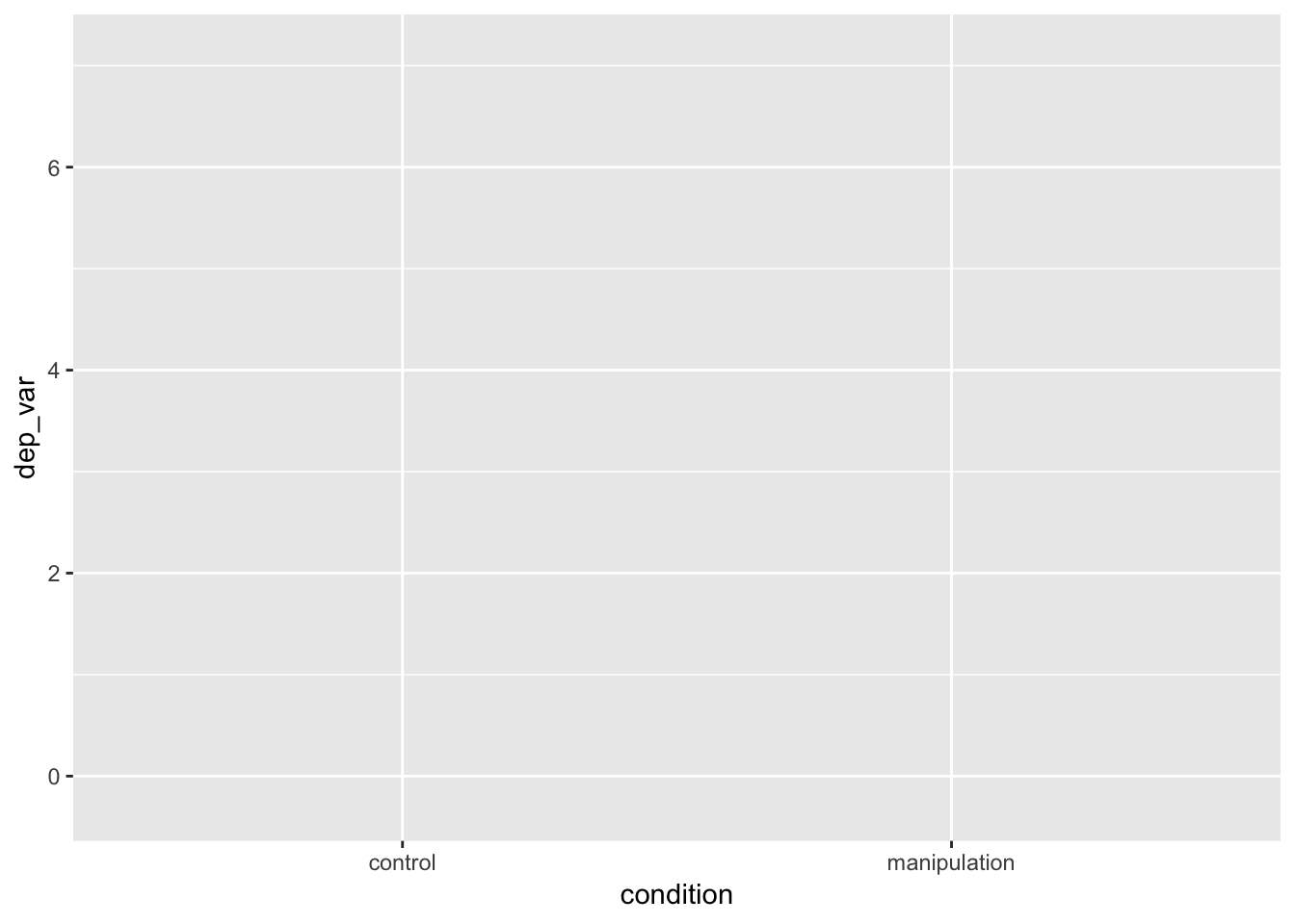
- Think of this like a blank canvas that we’re going to add pictures to or like a map of the ocean we’re going to add land mass to
Boxplot
- next, we add—yes, add, with a
+—a geom, a geometric element:geom_boxplot()- see help(geom_boxplot) for details
example_data %>%
  ggplot(mapping = aes(x = condition, y = dep_var)) +
  geom_boxplot()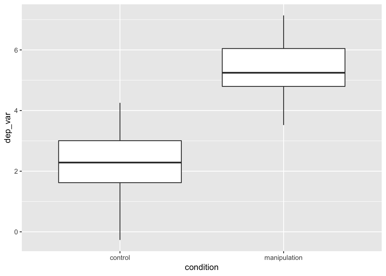
- Here’s emphasis: we started with a blank canvas, and we added a boxplot. All ggplots work this way: start with a base and add layers.
QQ-plots
- Below, we plot the sample quantiles of dep_var against the theoretical quantiles
- Useful for exploring the distribution of a variable
- see help(geom_qq) for details
example_data %>%
  ggplot(mapping = aes(sample = dep_var)) +
  geom_qq()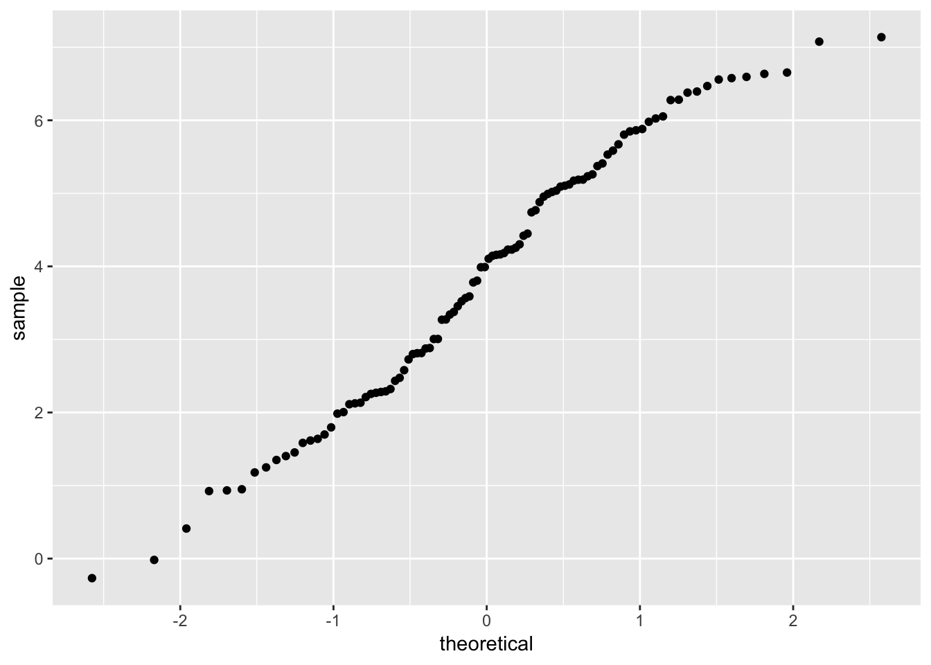
Means and 95% confidence intervals
- add a new aesthetic, fill, which will fill the geoms with different colors, depending on the variable (e.g., levels of categorical variables are assigned their own fill color)
stat_summary()does what its name suggests: it applies statistical summaries to your raw data to make the geoms (bars and error bars in our case below)- the width argument sets the width of the error bars.
- see help(stat_summary) for details
example_data %>%
  ggplot(mapping = aes(x = condition, y = dep_var, fill = condition)) +
  stat_summary(geom = "bar", fun.data = mean_cl_normal) +
  stat_summary(geom = "errorbar", fun.data = mean_cl_normal, width = 0.1)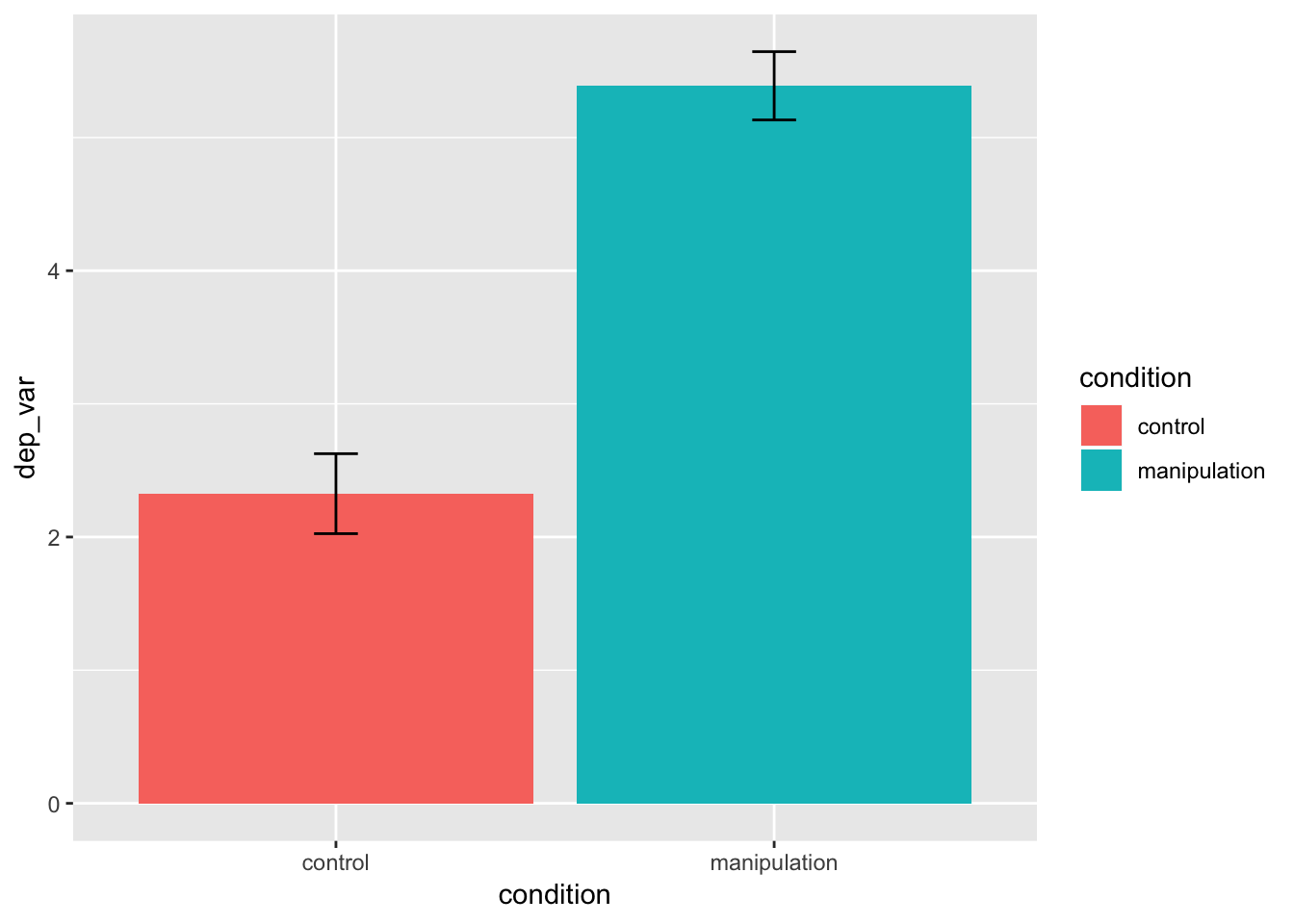
Scatterplots
- we add
geom_point()andgeom_smooth()below to add points to the scatterplot and fit a linear regression line with 95% confidence ribbons/bands around that line- see help(geom_point) and help(geom_smooth)for details
example_data %>%
  ggplot(mapping = aes(x = confound, y = dep_var)) +
  geom_point() +
  geom_smooth(method = "lm", se = TRUE)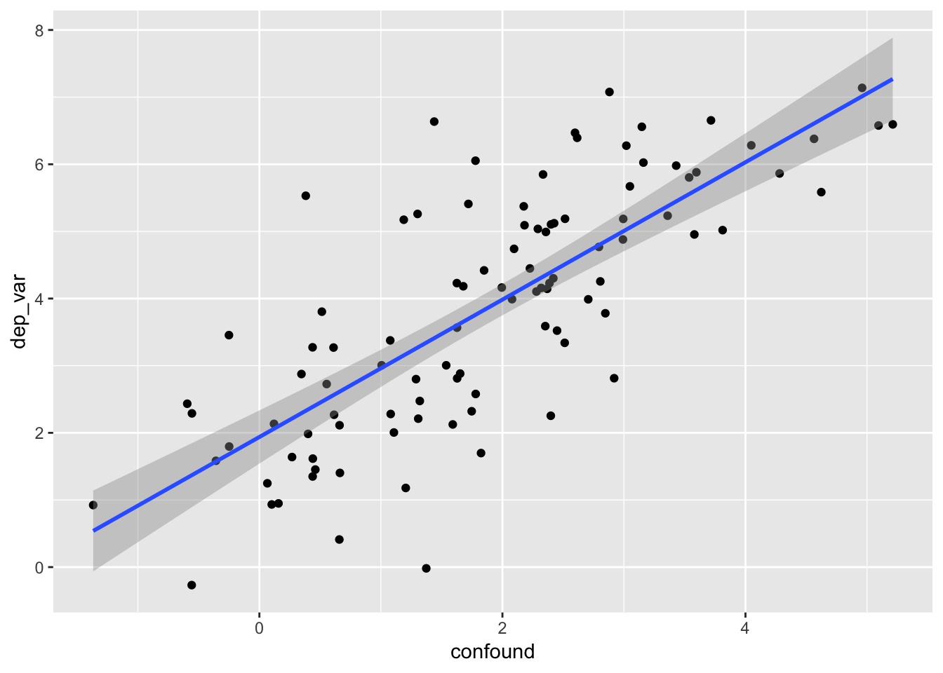
Descriptive statistics
describe(), help(describe)describeBy(), help(describeBy)
For whole sample
example_data %>%
  select(dep_var, dep_var_z, confound, confound_z) %>%
  describe()
## vars n mean sd median trimmed mad min max range skew
## dep_var 1 100 3.86 1.82 4.05 3.89 2.24 -0.27 7.14 7.41 -0.14
## dep_var_z 2 100 0.00 1.00 0.10 0.02 1.23 -2.26 1.80 4.06 -0.14
## confound 3 100 1.88 1.37 1.84 1.84 1.43 -1.37 5.21 6.58 0.17
## confound_z 4 100 0.00 1.00 -0.03 -0.03 1.04 -2.37 2.44 4.81 0.17
## kurtosis se
## dep_var -1.0 0.18
## dep_var_z -1.0 0.10
## confound -0.3 0.14
## confound_z -0.3 0.10By condition
The code below is a little confusing. First, we’re piping our subsetted tibble with only our four variables—dep_var and confound and their z-scored versions—into the first argument for the
describeBy()function. But we need to give data to the group argument, so then we just give it another subsetted tibble with only our grouping variable, condition.
example_data %>%
  select(dep_var, dep_var_z, confound, confound_z) %>%
  describeBy(group = example_data %>% select(condition))
##
## Descriptive statistics by group
## condition: control
## vars n mean sd median trimmed mad min max range skew
## dep_var 1 50 2.33 1.06 2.29 2.35 1.05 -0.27 4.26 4.52 -0.27
## dep_var_z 2 50 -0.84 0.58 -0.86 -0.82 0.58 -2.26 0.22 2.48 -0.27
## confound 3 50 0.96 0.99 0.83 0.94 1.05 -1.37 2.92 4.29 0.08
## confound_z 4 50 -0.67 0.72 -0.76 -0.68 0.77 -2.37 0.76 3.13 0.08
## kurtosis se
## dep_var -0.40 0.15
## dep_var_z -0.40 0.08
## confound -0.58 0.14
## confound_z -0.58 0.10
## --------------------------------------------------------
## condition: manipulation
## vars n mean sd median trimmed mad min max range skew
## dep_var 1 50 5.39 0.90 5.25 5.39 1.12 3.52 7.14 3.62 0.01
## dep_var_z 2 50 0.84 0.49 0.76 0.84 0.61 -0.18 1.80 1.98 0.01
## confound 3 50 2.80 1.04 2.56 2.73 0.80 0.38 5.21 4.83 0.44
## confound_z 4 50 0.67 0.76 0.50 0.63 0.59 -1.09 2.44 3.53 0.44
## kurtosis se
## dep_var -0.97 0.13
## dep_var_z -0.97 0.07
## confound -0.07 0.15
## confound_z -0.07 0.11Read in your own data
- .csv file:
read_csv()- .txt file:
read_delim()- SPSS .sav file:
read_sav()
SPSS
- see help(read_sav) for details
# path to where file lives on your computer
coffee_filepath <- "data/coffee.sav"

coffee_data <- read_sav(coffee_filepath)

# print coffee_data by just excecuting/running the name of the object
coffee_data
## # A tibble: 138 x 3
## image brand freq
## <dbl+lbl> <dbl+lbl> <dbl>
## 1 1 1 82
## 2 2 1 96
## 3 3 1 72
## 4 4 1 101
## 5 5 1 66
## 6 6 1 6
## 7 7 1 47
## 8 8 1 1
## 9 9 1 16
## 10 10 1 60
## # … with 128 more rowsCSV
- see help(read_csv) for details
# path to where file lives on your computer
coffee_filepath <- "data/coffee.csv"

coffee_data <- read_csv(coffee_filepath)
## Parsed with column specification:
## cols(
## image = col_double(),
## brand = col_double(),
## freq = col_double()
## )TXT
- see help(read_delim) for details
# path to where file lives on your computer
coffee_filepath <- "data/coffee.txt"

coffee_data <- read_delim(coffee_filepath, delim = " ")
## Parsed with column specification:
## cols(
## image = col_double(),
## brand = col_double(),
## freq = col_double()
## )Modeling your data
t.test(), help(t.test)
t.test(dep_var ~ condition, data = example_data)##
## Welch Two Sample t-test
##
## data: dep_var by condition
## t = -15.588, df = 95.663, p-value < 2.2e-16
## alternative hypothesis: true difference in means is not equal to 0
## 95 percent confidence interval:
## -3.453165 -2.673003
## sample estimates:
## mean in group control mean in group manipulation
## 2.325443 5.388527pairs.panels(), help(pairs.panels)
shows a scatter plot of matrices (SPLOM), with bivariate scatter plots below the diagonal, histograms on the diagonal, and the Pearson correlation above the diagonal (see ?pairs.panels).
example_data %>%
  select(dep_var, confound, age) %>%
  pairs.panels()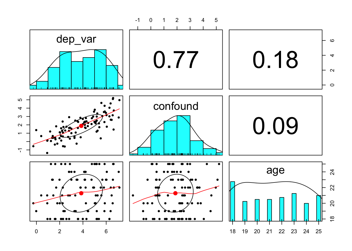
lm(), help(lm)
lm_fit <- lm(dep_var ~ condition + confound, data = example_data)

# print lm_fit by just excecuting/running the name of the object
lm_fit
##
## Call:
## lm(formula = dep_var ~ condition + confound, data = example_data)
##
## Coefficients:
## (Intercept) conditionmanipulation confound
## 1.8611 2.1710 0.4853summary(), help(summary)
summary(lm_fit)##
## Call:
## lm(formula = dep_var ~ condition + confound, data = example_data)
##
## Residuals:
## Min 1Q Median 3Q Max
## -2.54595 -0.60775 -0.04598 0.59644 1.90531
##
## Coefficients:
## Estimate Std. Error t value Pr(>|t|)
## (Intercept) 1.8611 0.1457 12.778 < 2e-16 ***
## conditionmanipulation 2.1710 0.2316 9.376 2.99e-15 ***
## confound 0.4853 0.0850 5.709 1.24e-07 ***
## ---
## Signif. codes: 0 '***' 0.001 '**' 0.01 '*' 0.05 '.' 0.1 ' ' 1
##
## Residual standard error: 0.8544 on 97 degrees of freedom
## Multiple R-squared: 0.7849, Adjusted R-squared: 0.7804
## F-statistic: 177 on 2 and 97 DF, p-value: < 2.2e-16Anova(), help(Anova)
Anova(lm_fit, type = "III")## Anova Table (Type III tests)
##
## Response: dep_var
## Sum Sq Df F value Pr(>F)
## (Intercept) 119.195 1 163.280 < 2.2e-16 ***
## condition 64.172 1 87.906 2.988e-15 ***
## confound 23.796 1 32.598 1.237e-07 ***
## Residuals 70.810 97
## ---
## Signif. codes: 0 '***' 0.001 '**' 0.01 '*' 0.05 '.' 0.1 ' ' 1Recommended Resources
- ReadCollegePDX (2015, October 19). Hadley Wickham “Data Science with R”. [YouTube]
- Robinson, D. (2017, July 05). Teach the tidyverse to beginners. Variance Explained. [.html]
- Wickham, H. (2014). Tidy data. Journal of Statistical Software, 59(10), 1-23. [.html]
- The tidyverse style guide [.html] by Hadley Wickham
- Wickham, H., & Grolemund, G. (2017). R for Data Science: Import, Tidy, Transform, Visualize, and Model Data. Sebastopol, CA: O’Reilly Media, Inc. [.html]
More advanced data wrangling and analysis techniques by psychologists, for psychologists
- R programming for research [.html], a workshop instructed by Nick Michalak and Iris Wang at the University of Michigan
More information about tidyverse and the psych package
R Studio Cheat Sheets
- RStudio Cheat Sheets [.html]
Nicholas M. Michalak
Data Scientist | Ph.D. Social Psychology
I study how both modern and evolutionarily-relevant threats affect how people perceive themselves and others.