Testing Between-Subjects Contrasts in R
Between-Subjects Factors
A between-subjects factor refers to independent groups that vary along some dimension. Put another way, a between-subjects factor assumes that each level of the factor represents an independent (i.e., not correlated) group of observations. For example, an experimental factor could represent 2 independent groups of participants who were randomly assigned to either a control or a treatment groupition. In this case, the between-subjects experimental factor assumes that measurements from both groups of participants are not correlated – they are independent.
What are contrasts?
Broadly, contrasts test focused research hypotheses. A contrast comprises a set of weights or numeric values that represent some comparison. For example, when comparing two experimental group means (i.e., control vs. treatment), you can apply weights to each group mean and then sum them up. This is the same thing as subtracting one group’s mean from the other’s.
Here’s a quick demonstration
# group means
control <- 5
treatment <- 3

# apply contrast weights and sum up the results
sum(c(control, treatment) * c(1, -1))
## [1] 2Model and Conceptual Assumptions for Linear Regression
- Correct functional form. Your model variables share linear relationships.
- No omitted influences. This one is hard: Your model accounts for all relevant influences on the variables included. All models are wrong, but how wrong is yours?
- Accurate measurement. Your measurements are valid and reliable. Note that unreliable measures can’t be valid, and reliable measures don’t necessairly measure just one construct or even your construct.
- Well-behaved residuals. Residuals (i.e., prediction errors) aren’t correlated with predictor variables or eachother, and residuals have constant variance across values of your predictor variables.
Some assumptions worded differently for ANOVA
- Homogenous group variances. Group variances are equal. In this case, you can think of group variance as the “average” difference from the group mean (differences are squared so that they are all positive). Link this to the well-behaved residuals assumption above. Residuals (i.e., prediction errors) should be equal across groups; remember that, in ANOVA, groups are predictors.
- Normally distributed group observations. Group observations come from normal distributions. Also link this to the well-behaved residuals assumption above. Residuals should come from a normal distribution too.
Libraries
library(tidyverse)
library(knitr)
library(AMCP)
Load data
From Chapter 5, Table 4 in Maxwell, Delaney, & Kelley (2018)
Fromhelp("C5T4"): “The following data consists of blood pressure measurements for six individuals randomly assigned to one of four groups. Our purpose here is to perform four planed contrasts in order to discern if group differences exist for the selected contrasts of interests.”
data("C5T4")

# add labels
C5T4 <- C5T4 %>% mutate(group_lbl = group %>% recode(`1` = "Drug Therapy", `2` = "Biofeedback", `3` = "Diet", `4` = "Combination"))
Print full dataset
C5T4 %>%
kable()| group | sbp | group_lbl |
|---|---|---|
| 1 | 84 | Drug Therapy |
| 1 | 95 | Drug Therapy |
| 1 | 93 | Drug Therapy |
| 1 | 104 | Drug Therapy |
| 1 | 99 | Drug Therapy |
| 1 | 106 | Drug Therapy |
| 2 | 81 | Biofeedback |
| 2 | 84 | Biofeedback |
| 2 | 92 | Biofeedback |
| 2 | 101 | Biofeedback |
| 2 | 80 | Biofeedback |
| 2 | 108 | Biofeedback |
| 3 | 98 | Diet |
| 3 | 95 | Diet |
| 3 | 86 | Diet |
| 3 | 87 | Diet |
| 3 | 94 | Diet |
| 3 | 101 | Diet |
| 4 | 91 | Combination |
| 4 | 78 | Combination |
| 4 | 85 | Combination |
| 4 | 80 | Combination |
| 4 | 81 | Combination |
| 4 | 76 | Combination |
Visualize relationships
It’s always a good idea to look at your data. Check some assumptions.
boxplots
Do variances look equal?
C5T4 %>%
  ggplot(mapping = aes(x = group_lbl, y = sbp, fill = group_lbl)) +
  geom_boxplot() +
  theme_bw() +
  theme(legend.position = "top")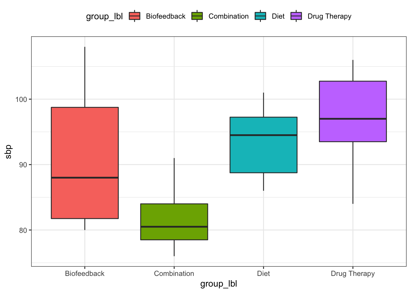
QQ-plots
Do observations look normal?
C5T4 %>%
  ggplot(mapping = aes(sample = sbp)) +
  geom_qq() +
  facet_wrap(facets = ~ group_lbl, scales = "free") +
  theme_bw()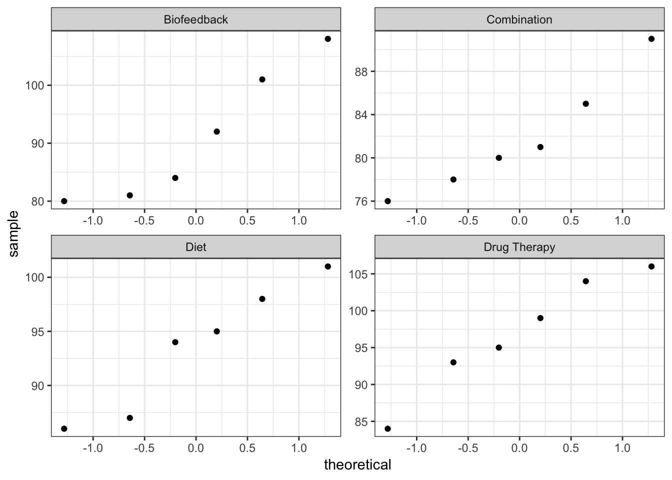
Define custom oneway function (similar to IBM SPSS’s ONEWAY command)
oneway <- function(dv, group, contrast, alpha = .05) {
  # -- arguments --
  # dv: vector of measurements (i.e., dependent variable)
  # group: vector that identifies which group the dv measurement came from
  # contrast: list of named contrasts
  # alpha: alpha level for 1 - alpha confidence level
  # -- output --
  # computes confidence interval and test statistic for a linear contrast of population means in a between-subjects design
  # returns a data.frame object
  # estimate (est), standard error (se), t-statistic (z), degrees of freedom (df), two-tailed p-value (p), and lower (lwr) and upper (upr) confidence limits at requested 1 - alpha confidence level
  # first line reports test statistics that assume variances are equal
  # second line reports test statistics that do not assume variances are equal

  # means, standard deviations, and sample sizes
  ms <- by(dv, group, mean, na.rm = TRUE)
  vars <- by(dv, group, var, na.rm = TRUE)
  ns <- by(dv, group, function(x) sum(!is.na(x)))

  # convert list of contrasts to a matrix of named contrasts by row
  contrast <- matrix(unlist(contrast), nrow = length(contrast), byrow = TRUE, dimnames = list(names(contrast), NULL))

  # contrast estimate
  est <- contrast %*% ms

  # welch test statistic
  se_welch <- sqrt(contrast^2 %*% (vars / ns))
  t_welch <- est / se_welch

  # classic test statistic
  mse <- anova(lm(dv ~ factor(group)))$"Mean Sq"[2]
  se_classic <- sqrt(mse * (contrast^2 %*% (1 / ns)))
  t_classic <- est / se_classic

  # if dimensions of contrast are NULL, nummer of contrasts = 1, if not, nummer of contrasts = dimensions of contrast
  num_contrast <- ifelse(is.null(dim(contrast)), 1, dim(contrast)[1])
  df_welch <- rep(0, num_contrast)
  df_classic <- rep(0, num_contrast)

  # makes rows of contrasts if contrast dimensions aren't NULL
  if(is.null(dim(contrast))) contrast <- t(as.matrix(contrast))

  # calculating degrees of freedom for welch and classic
  for(i in 1:num_contrast) {
    df_classic[i] <- sum(ns) - length(ns)
    df_welch[i] <- sum(contrast[i, ]^2 * vars / ns)^2 / sum((contrast[i, ]^2 * vars / ns)^2 / (ns - 1))
  }

  # p-values
  p_welch <- 2 * (1 - pt(abs(t_welch), df_welch))
  p_classic <- 2 * (1 - pt(abs(t_classic), df_classic))

  # 95% confidence intervals
  lwr_welch <- est - se_welch * qt(p = 1 - (alpha / 2), df = df_welch)
  upr_welch <- est + se_welch * qt(p = 1 - (alpha / 2), df = df_welch)
  lwr_classic <- est - se_classic * qt(p = 1 - (alpha / 2), df = df_classic)
  upr_classic <- est + se_classic * qt(p = 1 - (alpha / 2), df = df_classic)

  # output
  data.frame(contrast = rep(rownames(contrast), times = 2),
             equal_var = rep(c("Assumed", "Not Assumed"), each = num_contrast),
             est = rep(est, times = 2),
             se = c(se_classic, se_welch),
             t = c(t_classic, t_welch),
             df = c(df_classic, df_welch),
             p = c(p_classic, p_welch),
             lwr = c(lwr_classic, lwr_welch),
             upr = c(upr_classic, upr_welch))
}
Test contrasts (Maxwell & Dalaney, 2004, p. 207)
Drug Therapy vs. Biofeedback: 1, -1, 0, 0
Drug Therapy vs. Diet: 1, 0, -1, 0
Biofeedback vs. Diet: 0, 1, -1, 0
Drug Therapy, Biofeedback, and Diet vs. Combination: 1, 1, 1, -3
with(C5T4,
oneway(dv = sbp, group = group, contrast = list(dtVbf = c(1, -1, 0, 0),
                                                dtVd = c(1, 0, -1, 0),
                                                bfVd = c(0, 1, -1, 0),
                                                dtbfdVc = c(1, 1, 1, -3)), alpha = 0.05)
) %>%
kable()| contrast | equal_var | est | se | t | df | p | lwr | upr |
|---|---|---|---|---|---|---|---|---|
| dtVbf | Assumed | 5.833333 | 4.667559 | 1.2497609 | 20.000000 | 0.2258144 | -3.903025 | 15.569692 |
| dtVd | Assumed | 3.333333 | 4.667559 | 0.7141491 | 20.000000 | 0.4833872 | -6.403025 | 13.069692 |
| bfVd | Assumed | -2.500000 | 4.667559 | -0.5356118 | 20.000000 | 0.5981333 | -12.236358 | 7.236358 |
| dtbfdVc | Assumed | 35.833333 | 11.433139 | 3.1341641 | 20.000000 | 0.0052236 | 11.984223 | 59.682443 |
| dtVbf | Not Assumed | 5.833333 | 5.723732 | 1.0191485 | 8.947047 | 0.3348981 | -7.126340 | 18.793006 |
| dtVd | Not Assumed | 3.333333 | 4.083844 | 0.8162246 | 9.221906 | 0.4349481 | -5.871187 | 12.537854 |
| bfVd | Not Assumed | -2.500000 | 5.283622 | -0.4731602 | 7.507995 | 0.6495483 | -14.824442 | 9.824442 |
| dtbfdVc | Not Assumed | 35.833333 | 9.095481 | 3.9396853 | 13.288009 | 0.0016279 | 16.226946 | 55.439720 |
Interpretation
We found no sufficient evidence that, following treatment, those in the Drug Therapy condition had different blood pressure values, on average, than those in the Biofeedback condition, t(8.95) = 1.02, p = .335; that those in the Drug Therapy condition had different blood pressure values, on average, than those in the Diet condition, t(9.22) = 0.82, p = .435; or that those in the Biofeedback condition had different blood pressure values, on average, than those in the Diet condition, t(7.51) = -0.47, p = .650. However, we found evidence that, following treatment, those in the Drug Therapy, Biofeedback, and Diet conditions all together had higher blood pressure values, on average, than those in the Combination condition, b = 35.83, 95% CI [16.23, 55.44], t(13.29) = 3.95, p = .002.
A simulation
The correction for unequal equal variances Welch’s t-test may seem to have only trivial effects on the contrast test statistics, but the corrected test statistics maintain error rates (i.e., rejecting a true null 5% of the time) much better than the classic contrast test statistics when sample sizes and standard deviaitions are different. Moreover, when sample sizes and standard deviaitions are equal, the corrected test statistics give more or less the same results as the classic test statistics without sacrificing power in any practical sense. Below I simulate both extremes.
Generate simulation data
- Equal sample sizes and equal standard deviations
- Unequal sample sizes and unequal standard deviations
# set random seed so results can be reproduced
set.seed(7777)

# sample sizes for both conditions
ns1 <- c(50, 50, 50, 50); ns2 <- c(75, 25, 50, 50)

# means (only 1 set of group means)
ms <- c(4, 4, 4, 4)

# standard deviations for both conditions
sds1 <- c(1, 1, 1, 1); sds2 <- c(0.5, 1, 1, 1)

# g identifies which groups the data come from
g1 <- rep(rep(1:4, times = ns1), times = 10000); g2 <- rep(rep(1:4, times = ns2), times = 10000)

# k = simulation replicate
k <- rep(1:10000, each = 200)

# this code create a data.frame with every combination of k and g
simdat1 <- data.frame(k, g = g1); simdat2 <- data.frame(k, g = g2)
simdat1$y <- rnorm(n = ns1[simdat1$g], mean = ms[simdat1$g], sd = sds1[simdat1$g])
simdat2$y <- rnorm(n = ns2[simdat2$g], mean = ms[simdat2$g], sd = sds2[simdat2$g])
Define simulation tests function
In the function below, I test the interaction contrast as if the 4 groups came from a 2 x 2 factorial design (e.g., Aa = 1, Ab = -1, Ba = -1, Bb = 1).
simtest <- function(data) {
  # save output
  contout <- with(data, oneway(dv = y, group = g, contrast = list(cont1 = c(1, -1, -1, 1)), alpha = 0.05))

  # save classic two-tailed p-value
  p_classic <- contout[contout$equal_var == "Assumed", ]$p
  p_welch <- contout[contout$equal_var == "Not Assumed", ]$p

  # output
  cbind(p = c(p_classic, p_welch), welch = c(0, 1))
}
Generate test results (i.e., p-values)
simp1 <- unique(simdat1$k) %>%
  map_df(function(i) {
    simdat1 %>%
      filter(k == i) %>%
      simtest() %>%
      as_tibble()
  }) %>%
  mutate(cond = "Equal N & Equal SD", sig = as.numeric(p < .05))

simp2 <- unique(simdat2$k) %>%
  map_df(function(i) {
    simdat2 %>%
      filter(k == i) %>%
      simtest() %>%
      as_tibble()
  }) %>%
  mutate(cond = "Unequal N & Unequal SD", sig = as.numeric(p < .05))
Plot error rates
p < .05 should only occur 5% of the time
bind_rows(simp1, simp2) %>%
  group_by(cond, welch) %>%
  summarise(falsepos = mean(sig)) %>%
  mutate(welch = welch %>% recode(`0` = "Classic ANOVA", `1` = "Welch Correction")) %>%
  ggplot(mapping = aes(x = cond, y = falsepos, fill = welch)) +
  geom_bar(stat = "identity", position = position_dodge(0.9)) +
  geom_hline(yintercept = 0.05, color = "red") +
  scale_y_continuous(breaks = seq(0, 0.1, 0.01)) +
  theme_bw() +
  theme(legend.position = "top")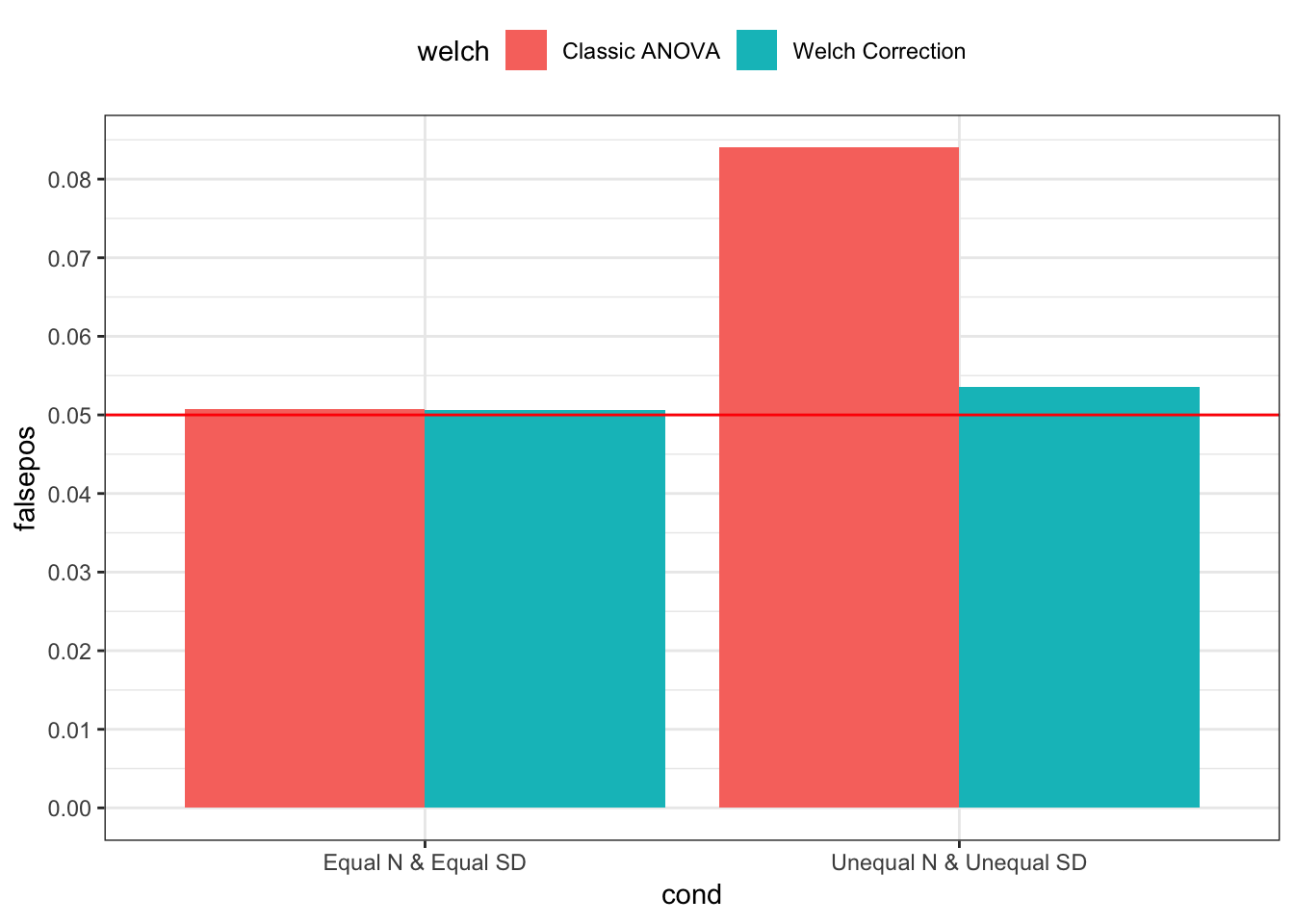
Interpretation
Above, I generated 10,000 sets of 4 group sample values whose true means were not different, and I tested the interaction contrast on each set (i.e., 2 x 2 factorial ANOVA interaction contrast). Like I described above, when sample sizes and standard deviaitions were equal, both contrast test statistics give practically the same results, on average, but when sample sizes and standard deviaitions were different – in this case, one group had a larger sample size and a smaller true standard deviation – the classic test statistics resulted in false positives over 8% of the time; the corrected test statistics resulted in false positives only 5% of the time.
Resources
- Bonett, D. G. (2008). Confidence intervals for standardized linear contrasts of means. Psychological Methods, 13(2), 99-109.
- Bonett, D. G. (2009). Meta-analytic interval estimation for standardized and unstandardized mean differences. Psychological Methods, 14(3), 225-238.
- Maxwell, S. E., Delaney, H. D., & Kelley, K. (2018). Designing experiments and analyzing data: A model comparison perspective (3rd ed.). Routledge.
- DESIGNING EXPERIMENTS AND ANALYZING DATA includes computer code for analyses from their book, Shiny apps, and more.
- Wondra, J.D., & Gonzalez, R. (In prep). Use Welch’s t Test to Compare the Means of Independent Groups. Unpublished Manuscript.
General word of caution
Above, I listed resources prepared by experts on these and related topics. Although I generally do my best to write accurate posts, don’t assume my posts are 100% accurate or that they apply to your data or research questions. Trust statistics and methodology experts, not blog posts.
Nicholas M. Michalak
Data Scientist | Ph.D. Social Psychology
I study how both modern and evolutionarily-relevant threats affect how people perceive themselves and others.