Using Principal Components or Common Factor Analysis in Social Psychology
Multidimensional Scaling, the precursor to Principal Components Analysis, Common Factor Analysis, and related techniques
Multidimensional scaling is an exploratory technique that uses distances or disimilarities between objects to create a multidimensional representation of those objects in metric space. In other words, multidimensional scaling uses data about the distance (e.g., miles between cities) or disimilarity (e.g., how (dis)similar are apples and tomatoes?) among a set of objects to “search” for some metric space that represents those objects and their relations to each other. Metric space is a fancy term for a set of objects and some metric that satisfy a list of axioms.
Here is one way to represent the distance (d) axioms:
- \[d_{ij} > d_{ii} = 0 \text{, for } i \neq j.\]
- \[d_{ij} = d_{ji}.\]
- \[d_{ij} \leq d_{ik} + d_{kj}.\]
Here is one way to represent the similarity (s) axioms:
- \[s_{ii} > s_{ij}.\]
- \[s_{ij} = s_ji.\]
- \[\text{a large } s_{ij} \text{ implies } d_{ik} \approx d_{kj}.\]
If you’re familiar with the Pythagorean Theorem \[c = \sqrt{a^2 + b^2}\], and you have a sense of what “similar” means, then these axioms should be intutuive to you. With regard to Multidimensional Scaling, the big idea here is that the data and the axioms constrain the solution you get. For example, if you’re making a map of U.S. cities—and you want an accurate map of the cities—then including 100,000 cities in your analysis will place more constraints on your solution than including 10 cities. More contraints in this case will give you a better picture of 10 cities and their relation to each other (e.g., New York is north of Miami) than fewer constraints.
This should be more clear in the example below.
Install packages and/or load libraries
I’ll use these packages throughout this post.
# install.packages("tidyverse")
# install.packages("knitr")
# install.packages("maps")
# install.packages("psych")
# install.packages("MASS")

library(tidyverse)
library(knitr)
library(maps)
library(psych)
library(MASS)

# use select from dplyr
select <- dplyr::select
Data
help("UScitiesD")
“UScitiesD gives “straight line” distances between 10 cities in the US.”
help(kable)converts amatrixordata.frameinto a simple but pretty Markdown table
UScitiesD %>%
  as.matrix() %>%
kable()| Atlanta | Chicago | Denver | Houston | LosAngeles | Miami | NewYork | SanFrancisco | Seattle | Washington.DC | |
|---|---|---|---|---|---|---|---|---|---|---|
| Atlanta | 0 | 587 | 1212 | 701 | 1936 | 604 | 748 | 2139 | 2182 | 543 |
| Chicago | 587 | 0 | 920 | 940 | 1745 | 1188 | 713 | 1858 | 1737 | 597 |
| Denver | 1212 | 920 | 0 | 879 | 831 | 1726 | 1631 | 949 | 1021 | 1494 |
| Houston | 701 | 940 | 879 | 0 | 1374 | 968 | 1420 | 1645 | 1891 | 1220 |
| LosAngeles | 1936 | 1745 | 831 | 1374 | 0 | 2339 | 2451 | 347 | 959 | 2300 |
| Miami | 604 | 1188 | 1726 | 968 | 2339 | 0 | 1092 | 2594 | 2734 | 923 |
| NewYork | 748 | 713 | 1631 | 1420 | 2451 | 1092 | 0 | 2571 | 2408 | 205 |
| SanFrancisco | 2139 | 1858 | 949 | 1645 | 347 | 2594 | 2571 | 0 | 678 | 2442 |
| Seattle | 2182 | 1737 | 1021 | 1891 | 959 | 2734 | 2408 | 678 | 0 | 2329 |
| Washington.DC | 543 | 597 | 1494 | 1220 | 2300 | 923 | 205 | 2442 | 2329 | 0 |
Represent the distance matrix with colors
- Convert the distance object into a
data.frame.
- Restructure the
data.frameso each distance value gets its own row, and each distance value corresponds to two city names (even cities paired with themselves, so distance = 0).
- Plot the distance values on tiles that are colored by the size of the distance.
UScitiesD %>%
  as.matrix() %>%
  as.data.frame() %>%
  mutate(city1 = rownames(.)) %>%
  gather(key = city2, value = distance, -city1) %>%
  ggplot(mapping = aes(x = city1, y = city2, fill = distance, label = distance)) +
  geom_tile() +
  geom_text() +
  scale_fill_gradient2() +
  theme(axis.text.x = element_text(angle = 90, hjust = 1))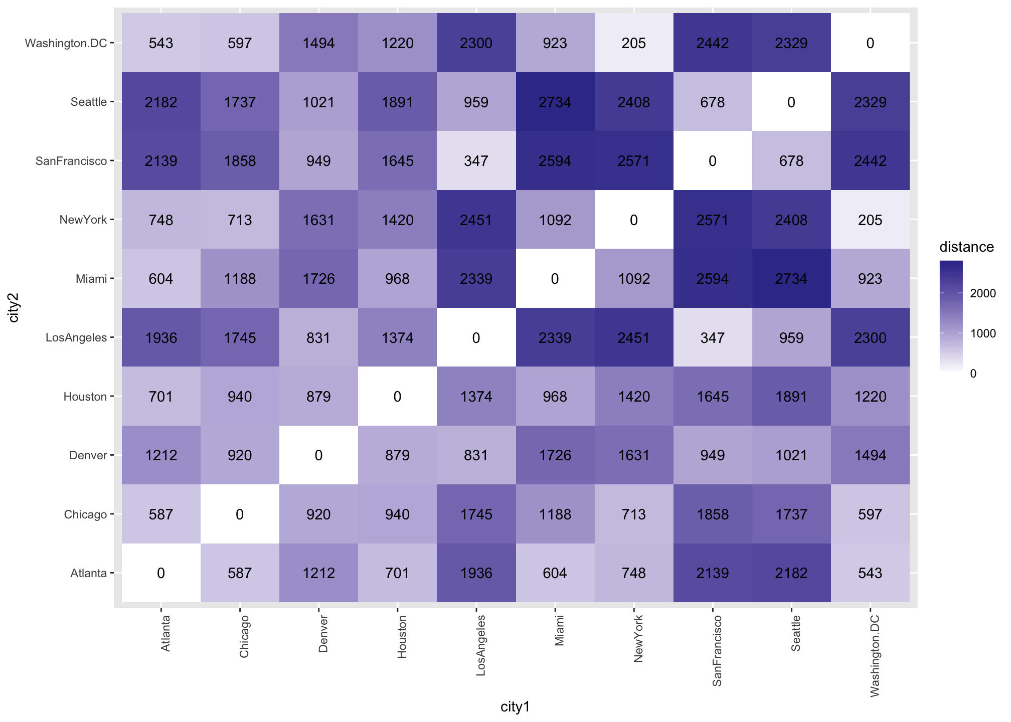
Interpretation
Darker tiles index that two cities are relatively far apart, and lighter tiles index that two cities are relatively close together (e.g., white tiles = a city is right next to itself)
Metric Multidimensional Scaling (2-dimensions, like a map)
help(cmdscale)
“Classical multidimensional scaling (MDS) of a data matrix. Also known as principal coordinates analysis (Gower, 1966).”
# give it distance values and number of dimensions
# also ask for the function to output eigenvalues
cmdscale.fit1 <- cmdscale(UScitiesD, k = 2, eig = TRUE)
Plot eigenvalues sorted by size (i.e., screeplot)
You can use eigenvalues to give you a sense of how many dimensions can capture most of the information from original data. A “big” eigenvalue means a lot of information is contained in a given dimension. You can tell how big the eigenvalues are by looking a a plot of the digenvalues sorted by size. Analysts typically determine the number of dimensions to use by counting eigenvalues from left to right until the pattern of points flattens out (i.e., there is little leftover information contained in the remaining dimensions).
tibble(index = 1:length(cmdscale.fit1$eig),
       eigenvalue = cmdscale.fit1$eig) %>%
  ggplot(mapping = aes(x = index, y = eigenvalue)) +
  geom_line() +
  geom_point() +
  scale_y_continuous(labels = scales::comma)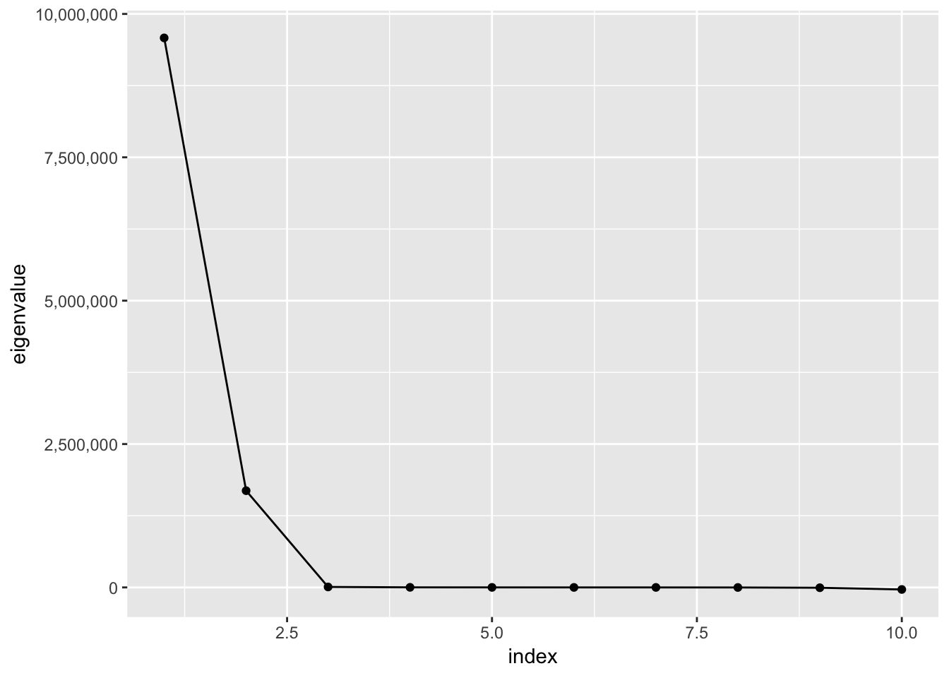
Interpretation
Because the lines stop dropping after 2-3 points, this suggest most of the information can be “captured” by 2-3 dimensions. To make a plot easier to interpret, I already asked for 2 dimensions.
Store points from the fitted configuration/solution in a tibble data.frame
The first and second dimension are stored as columns in the
pointsobject from thecmdscalefunction
cmdscale.data <- tibble(city = rownames(cmdscale.fit1$points),
                        dimension1 = cmdscale.fit1$points[, 1],
                        dimension2 = cmdscale.fit1$points[, 2])
Plot the solution
Note that I asked ggplot2 to plot the negative dimension scores to make the plot more interpretable compared to a map of the U.S. (i.e., real life)
cmdscale.data %>%
  ggplot(mapping = aes(x = -dimension1, y = -dimension2, label = city)) +
  geom_point() +
  geom_label(nudge_y = 100)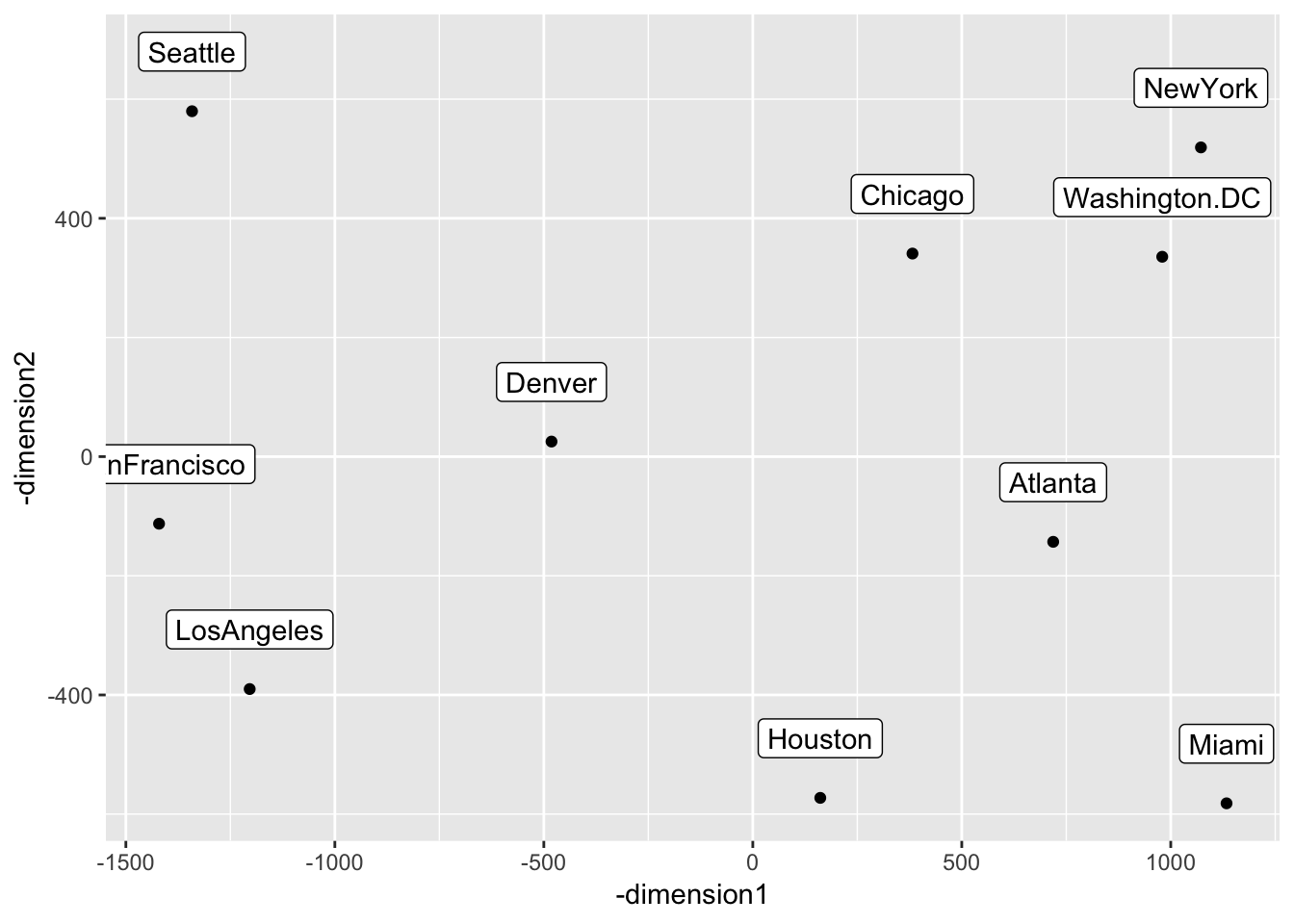
Compare the solution above to a map of the U.S. below
Because we only used pairwise distances among ten U.S. cities, the solution imperfectly represented real relations among these cities. For example, Miami seems to be in the right spot on the “Southeastern quadrant” of the plot, it seems to sit on almost a horizontal line with Houston; in real life, Houston is northwest of Miami, not directly west like the solution implies.
map_data("state") %>%
  ggplot(mapping = aes(x = long, y = lat, group = group)) +
  geom_polygon(fill = "white", colour = "black") +
  coord_quickmap()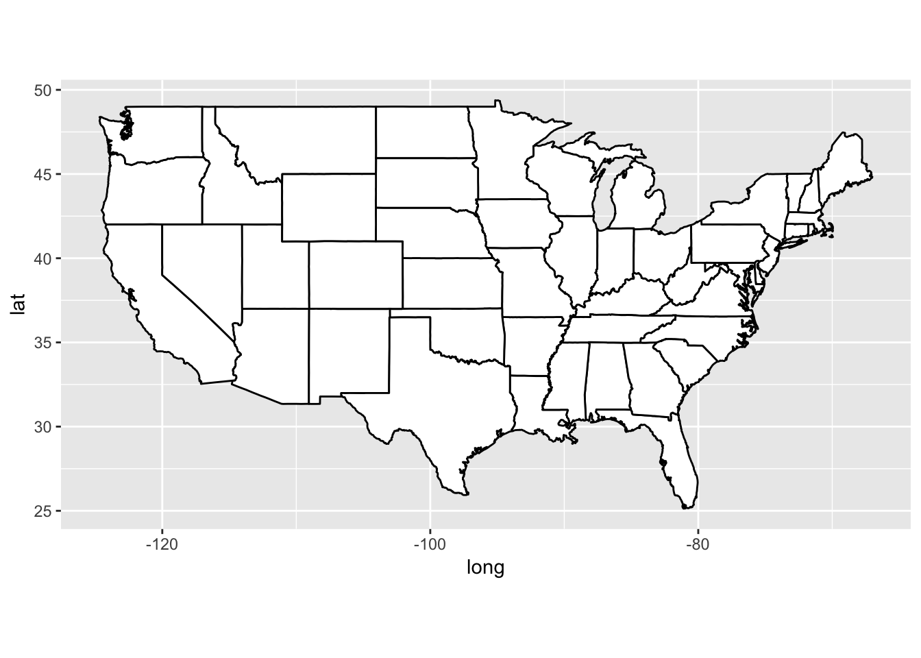
Principal Components and Common Factor Anlayses are special cases of Multidimensional Scaling
The major difference between Multidimensional Scaling and Principal Components and Common Factor Anlayses is that Multidimensional Scaling uses distances and (dis)similarity matrices and Principal Components and Common Factor Anlayses use covariance and correlation matrices. But all these techniques share common issues:
- How do you collect data (e.g., (dis)simlarities between items, likert responses to a question)
- How do you rotate the solution?
- What else can you measure to help you intepret the solution?
Principal Components and Common Factor Anlayses have a potentially pesky drawback: Whereas distance and (dis)similarities are more “direct” measures (e.g., asking participants to rate similarity doesn’t impose any particular psychological dimension on their judgments), likert-based questions may only indirectly get at which dimensions participants actually use to make judgments; these kinds of questions assume participants use the dimensions provided by the researcher. Keep this in mind as I walk through Principal Components and Common Factor Anlayses below.
Measuring variables we can’t observe
If we think psychological constructs like extraversion, social dominance orientation, or depression exist, then we should be able to measure them. We can’t measure these constructs directly like we can measure blood pressure or light absorption. But we can ask people questions that we believe index parts of what we mean by, say, extroversion (e.g., outgoing, sociable, acts like a leader). The questions we ask make up our measurement “test” (e.g., like a test of extroversion), and the scores on our test comprise two parts: truth and error (random or systematic). In other words, unobservable psychological constructs and error can explain the scores we can observe from the tests we administer. This is the gist of classical test theory.
Partitioning variance
A factor analysis models the variability in item responses (e.g., responses to questions on a test). Some of that variability can be explained by the relationship between items; some can be explained by what is “special” about the items; and some can be explained by error, random or systematic.
Common Variance
Common variance refers to variability shared among the items (i.e., what can be explained by inter-item correlations)
Communality
Communality (h2) is one definition of common variance and can take values between 0 and 1: h2 = 0 means no observed variability can be explained, and 1 means all observed variability can be explained.
Unique Variance (u2)
Unique variance refers to not-common variance. It has two parts: specific and error.
Specific Variance
Specific variance refers to variance explained by “special” parts of particular items. For example, one of the extraversion items from the HEXACO asks whether respondents agree with the item, “Am usually active and full of energy.” It’s possible some of the variability in agreement to this item comes from people who conider themselves active because they exercise a lot or active because they’re talking to people a lot (i.e., physically active vs. social active).
Error Variance
Error variance refers to any variability that can’t be explained by common or specific variance. For example, people might respond differently because they just received a text message. Note that it’s difficult to distinguish specific variance from error variance unless people take the same test at least 2 times. This would allow you to look for response patterns that emerge across testing contexts that can’t be explained by what’s common among the questions.
What’s the difference between Principal Components Analysis and Common Factor Analysis?
The major difference in these techniques boils down to error: Whereas the Principal Components model assumes that all variance is common variance, the Common Factor model partitions variance into common and unique variance (which includes error). Another way to think about the difference is that the Principal Components model tries to explain as much variance as possible with a small number of components, and Common Factor model tries to explain the shared relationships among the items with a small number of factors after setting aside what is not shared (i.e., the item-specific parts and the error parts). Below, I demonstrate the differences in how these two techniques account for variance in a sample of Big Five Inventory questions.
Big Five Inventory
help(bfi)andhelp(bfi.dictionary)
“The first 25 items are organized by five putative factors: Agreeableness, Conscientiousness, Extraversion, Neuroticism, and Opennness.”
“The item data were collected using a 6 point response scale: 1 Very Inaccurate 2 Moderately Inaccurate 3 Slightly Inaccurate 4 Slightly Accurate 5 Moderately Accurate 6 Very Accurate”
Sample Questions
Note that some items are negatively worded (i.e., response to those questions run opposite to the theoretical trait). I’m going to mostly ignore that in the demonstrations below because it’s not important for understanding.
bfi.dictionary %>%
  slice(-c(26, 27, 28)) %>%
  select(Item, Big6, Keying) %>%
kable()| Item | Big6 | Keying |
|---|---|---|
| Am indifferent to the feelings of others. | Agreeableness | -1 |
| Inquire about others’ well-being. | Agreeableness | 1 |
| Know how to comfort others. | Agreeableness | 1 |
| Love children. | Agreeableness | 1 |
| Make people feel at ease. | Agreeableness | 1 |
| Am exacting in my work. | Conscientiousness | 1 |
| Continue until everything is perfect. | Conscientiousness | 1 |
| Do things according to a plan. | Conscientiousness | 1 |
| Do things in a half-way manner. | Conscientiousness | -1 |
| Waste my time. | Conscientiousness | -1 |
| Don’t talk a lot. | Extraversion | -1 |
| Find it difficult to approach others. | Extraversion | -1 |
| Know how to captivate people. | Extraversion | 1 |
| Make friends easily. | Extraversion | 1 |
| Take charge. | Extraversion | 1 |
| Get angry easily. | Emotional Stability | -1 |
| Get irritated easily. | Emotional Stability | -1 |
| Have frequent mood swings. | Emotional Stability | -1 |
| Often feel blue. | Emotional Stability | -1 |
| Panic easily. | Emotional Stability | -1 |
| Am full of ideas. | Openness | 1 |
| Avoid difficult reading material. | Openness | -1 |
| Carry the conversation to a higher level. | Openness | 1 |
| Spend time reflecting on things. | Openness | 1 |
| Will not probe deeply into a subject. | Openness | -1 |
Correlation matrix
bfi %>%
  select(A1, A2, A3, A4, A5, C1, C2, C3, C4, C5, E1, E2, E3, E4, E5, N1, N2, N3, N4, N5, O1, O2, O3, O4, O5) %>%
  cor(use = "pairwise.complete.obs") %>%
  round(2) %>%
  as.data.frame() %>%
  mutate(item1 = rownames(.)) %>%
  gather(key = item2, value = r, -item1) %>%
  ggplot(mapping = aes(x = item1, y = item2, fill = r, label = r)) +
  geom_tile() +
  geom_text() +
  scale_fill_gradient2() +
  theme(axis.text.x = element_text(angle = 90, hjust = 1))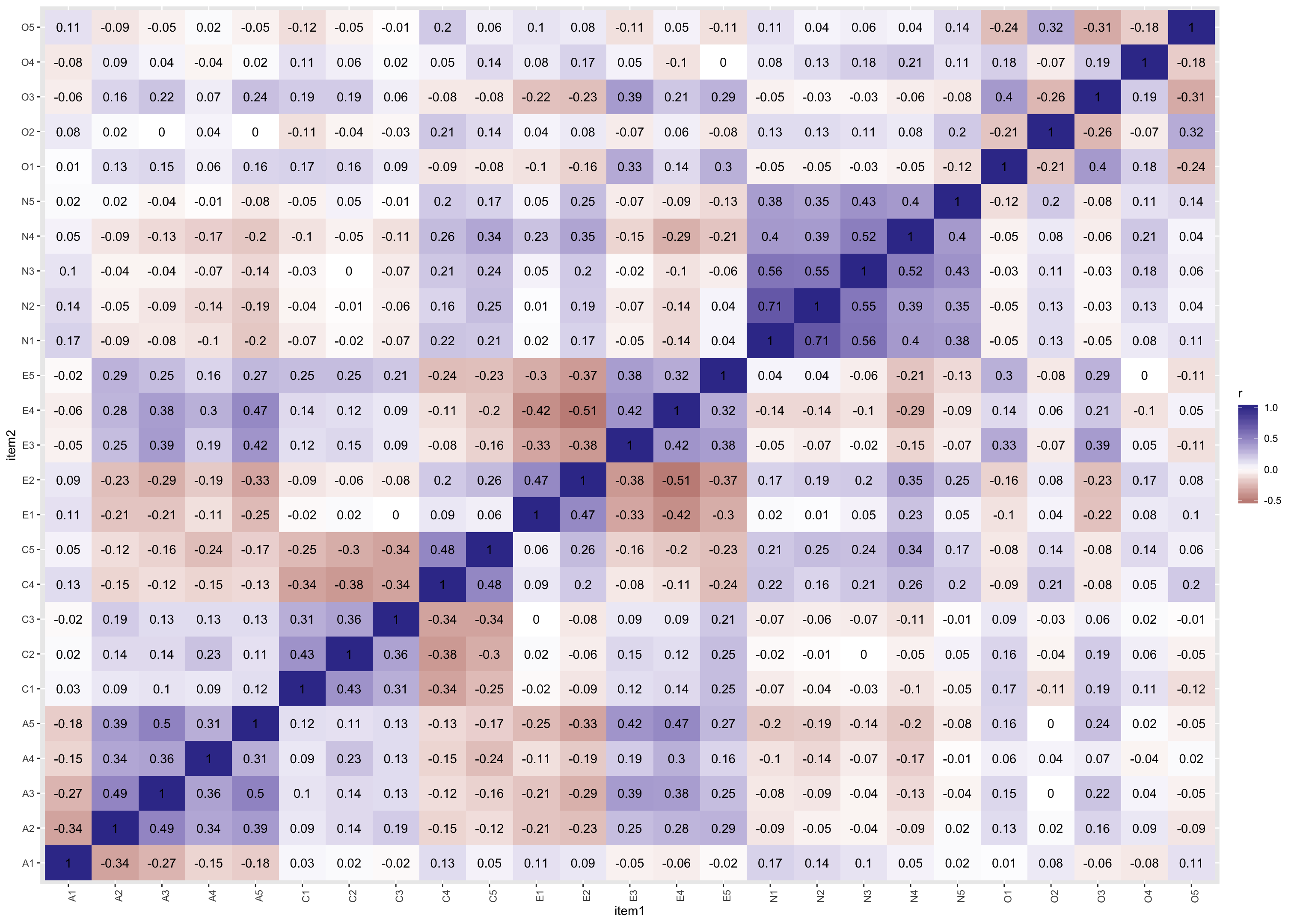
Interpretation
Darker purple tiles index more positive correlations, and darker red tiles index more negative correlations. Notice that 5 x 5 boxes of darker colors (i.e., more purple or more red, less white) emerge among similarly labeled items (i.e., the A items correlate more with A items than with C items or with O items)
Histograms
bfi %>%
  select(A1, A2, A3, A4, A5, C1, C2, C3, C4, C5, E1, E2, E3, E4, E5, N1, N2, N3, N4, N5, O1, O2, O3, O4, O5) %>%
  gather(key = variable, value = response) %>%
  ggplot(mapping = aes(x = response)) +
  geom_histogram(binwidth = 1, color = "white") +
  facet_wrap(facets = ~ variable)
## Warning: Removed 508 rows containing non-finite values (stat_bin).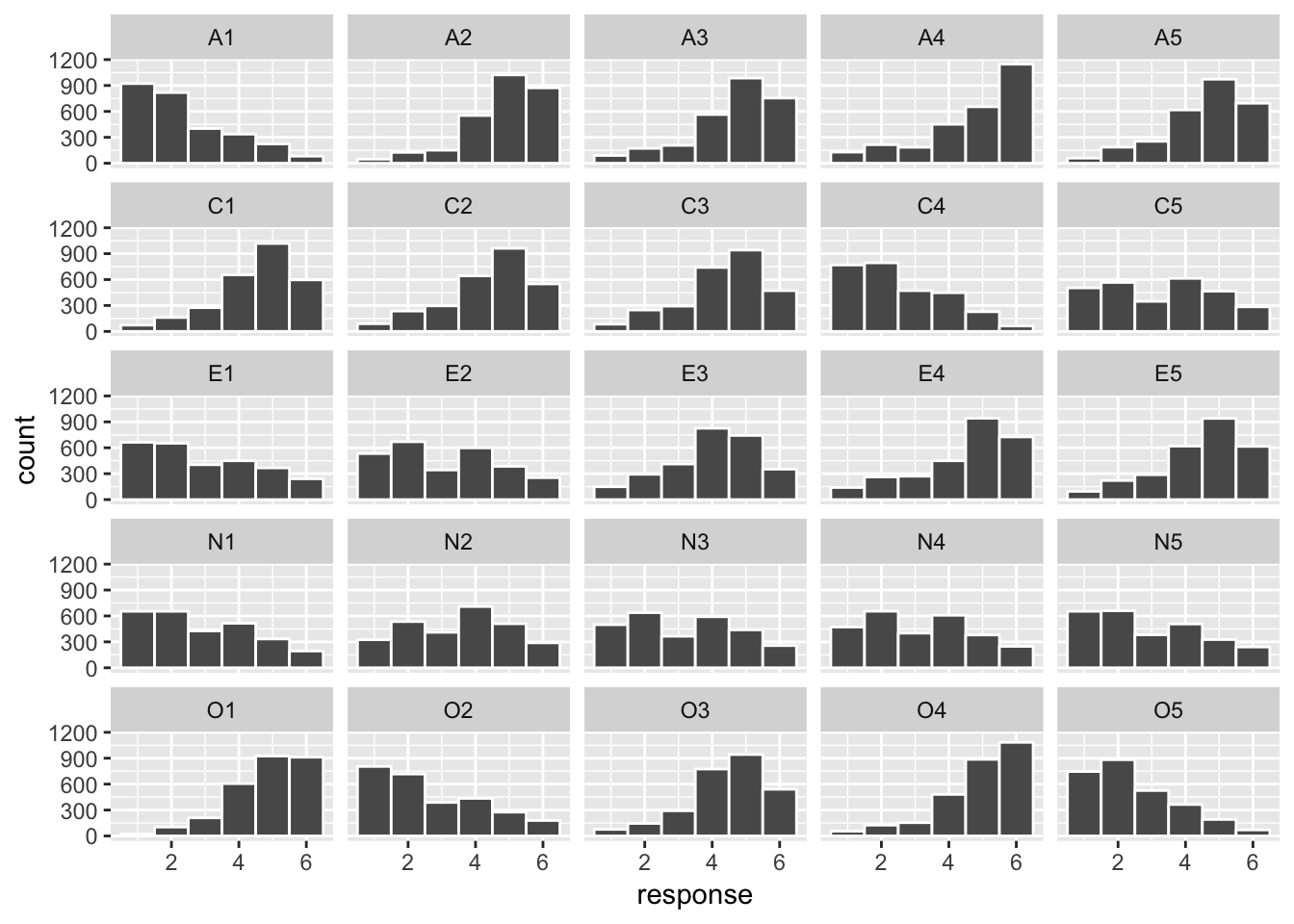
Interpretation
Each plot represents a histogram for a specific item. Bigger bars mean more participants gave that response. Notice that items vary in their response distributions (e.g., some items receive higher agreement than others, and some items receive more spread out agreement responses)
Parallel Analysis
help(fa.parallel)
“One way to determine the number of factors or components in a data matrix or a correlation matrix is to examine the “scree” plot of the successive eigenvalues. Sharp breaks in the plot suggest the appropriate number of components or factors to extract. “Parallel” analyis is an alternative technique that compares the scree of factors of the observed data with that of a random data matrix of the same size as the original.”
bfi %>%
  select(A1, A2, A3, A4, A5, C1, C2, C3, C4, C5, E1, E2, E3, E4, E5, N1, N2, N3, N4, N5, O1, O2, O3, O4, O5) %>%
  fa.parallel(fm = "minres", fa = "both")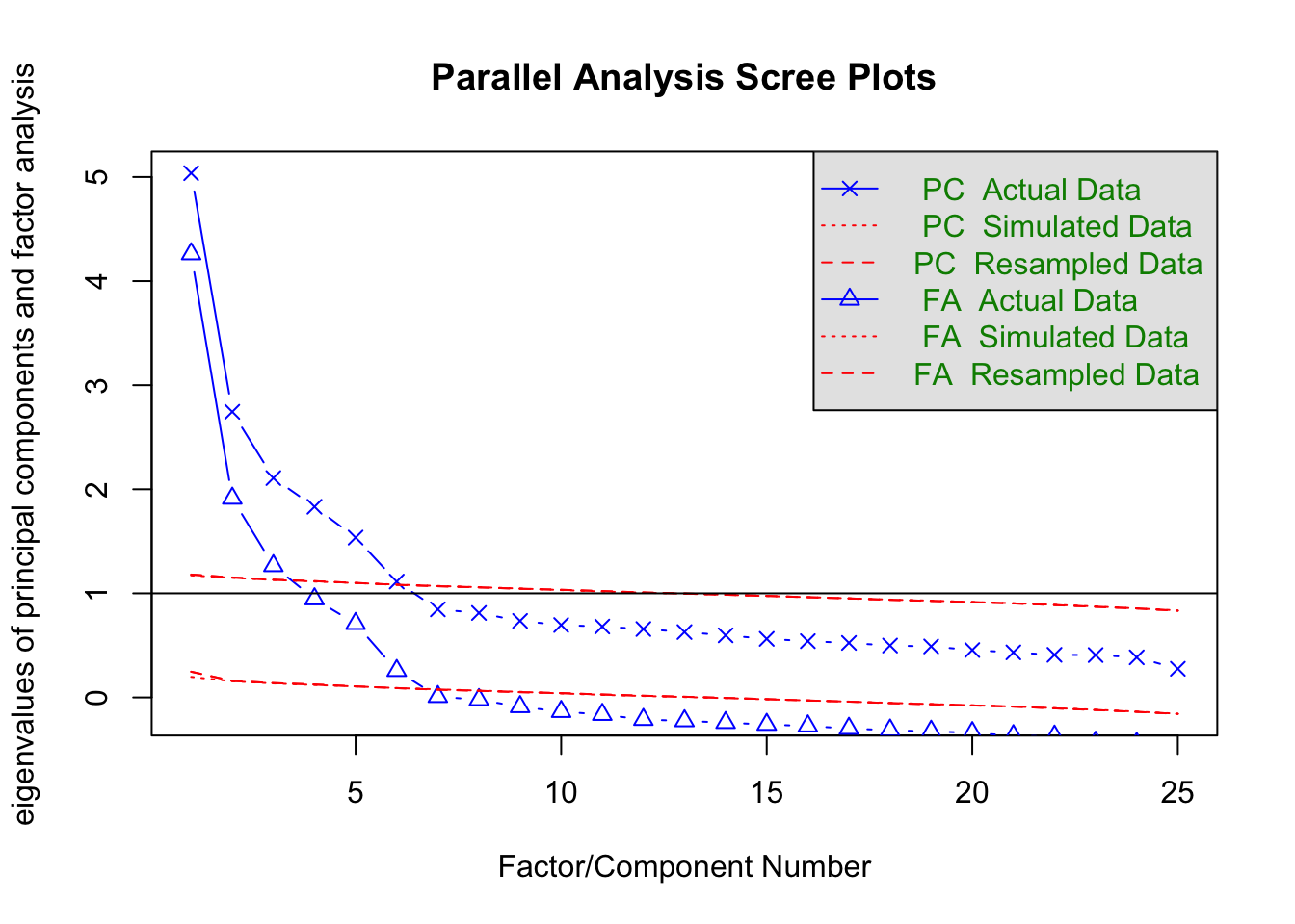
## Parallel analysis suggests that the number of factors = 6 and the number of components = 6Interpretation
As in the example from Multidimensional Scaling, one can artfully select how many dimensions to extract based on when the lines in these plots stop falling so precipitously. As an added benefit of parallel analysis, you can use the red lines to compare the eigenvalues to what you would expect from random data generated from the same number of items. William Revelle the package developer suggests using the plot of triangles (the common factor based eigenvalues). The output tells you how many factors you could extract based on where the blue lines cross the red dotted lines.
Principal Components Analysis
Save only the 25 items from the test (ignore reverse-worded items)
bfi25 <- bfi %>%
  select(A1, A2, A3, A4, A5, C1, C2, C3, C4, C5, E1, E2, E3, E4, E5, N1, N2, N3, N4, N5, O1, O2, O3, O4, O5)
Extract 5 components even though the parallel analysis suggested 6
Deciding how many components to extract should balance meaning with statistics-based heuristics or cutoffs. Extracting 5 components makes sense given previous research and theory on the 5 factors of personality, and, based on the screeplot, 5 components capture a lot of variance. Varimax rotation finds a solution that maximizes the variance captured by the components, which results in components that as much variance as possible for some items and almost no variance for other items (i.e., big loadings for some items, and small loadings for others). Importantly, the varimax solution effectively assumes components are uncorrelated.
principal(bfi25, nfactors = 5, rotate = "varimax") %>%
  print(sort = TRUE)
## Principal Components Analysis
## Call: principal(r = bfi25, nfactors = 5, rotate = "varimax")
## Standardized loadings (pattern matrix) based upon correlation matrix
## item RC2 RC1 RC3 RC5 RC4 h2 u2 com
## N1 16 0.79 0.07 -0.04 -0.21 -0.08 0.69 0.31 1.2
## N3 18 0.79 -0.04 -0.06 -0.03 0.00 0.63 0.37 1.0
## N2 17 0.79 0.04 -0.03 -0.19 -0.02 0.66 0.34 1.1
## N4 19 0.65 -0.34 -0.17 0.02 0.09 0.57 0.43 1.7
## N5 20 0.63 -0.16 -0.01 0.15 -0.17 0.48 0.52 1.4
## E2 12 0.27 -0.72 -0.07 -0.08 -0.02 0.60 0.40 1.3
## E4 14 -0.10 0.70 0.09 0.28 -0.12 0.61 0.39 1.5
## E1 11 0.04 -0.68 0.09 -0.07 -0.05 0.48 0.52 1.1
## E3 13 0.04 0.63 0.07 0.24 0.26 0.53 0.47 1.7
## E5 15 0.05 0.58 0.34 0.04 0.20 0.50 0.50 1.9
## C2 7 0.11 0.04 0.74 0.10 0.09 0.58 0.42 1.1
## C3 8 -0.01 0.00 0.67 0.13 -0.04 0.47 0.53 1.1
## C4 9 0.28 -0.04 -0.67 -0.05 -0.12 0.54 0.46 1.4
## C1 6 0.03 0.07 0.65 -0.01 0.21 0.47 0.53 1.2
## C5 10 0.33 -0.17 -0.62 -0.05 0.06 0.52 0.48 1.7
## A2 2 0.03 0.21 0.13 0.71 0.07 0.57 0.43 1.3
## A3 3 0.01 0.35 0.09 0.68 0.05 0.59 0.41 1.6
## A1 1 0.16 0.13 0.08 -0.63 -0.13 0.46 0.54 1.4
## A5 5 -0.12 0.44 0.08 0.56 0.04 0.54 0.46 2.1
## A4 4 -0.06 0.19 0.26 0.53 -0.17 0.41 0.59 2.0
## O5 25 0.12 0.01 -0.04 -0.03 -0.68 0.48 0.52 1.1
## O3 23 0.04 0.36 0.08 0.11 0.64 0.55 0.45 1.7
## O2 22 0.23 0.03 -0.09 0.11 -0.59 0.43 0.57 1.4
## O1 21 0.02 0.28 0.13 0.02 0.59 0.44 0.56 1.5
## O4 24 0.28 -0.24 -0.02 0.24 0.50 0.44 0.56 2.6
##
## RC2 RC1 RC3 RC5 RC4
## SS loadings 3.18 3.09 2.56 2.32 2.11
## Proportion Var 0.13 0.12 0.10 0.09 0.08
## Cumulative Var 0.13 0.25 0.35 0.45 0.53
## Proportion Explained 0.24 0.23 0.19 0.17 0.16
## Cumulative Proportion 0.24 0.47 0.67 0.84 1.00
##
## Mean item complexity = 1.5
## Test of the hypothesis that 5 components are sufficient.
##
## The root mean square of the residuals (RMSR) is 0.06
## with the empirical chi square 5469.42 with prob < 0
##
## Fit based upon off diagonal values = 0.92# plot
principal(bfi25, nfactors = 5, rotate = "varimax") %>%
fa.diagram(sort = TRUE, errors = TRUE)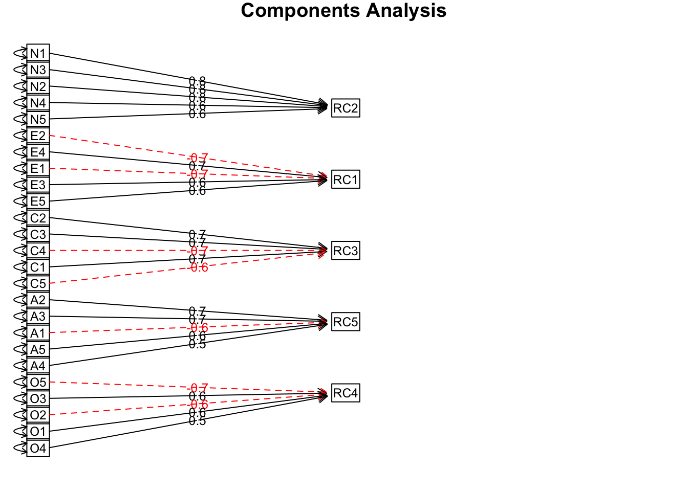
Interpretation
The component diagram gives you a big picture sense of the solution: there are 5 components, and the items vary in how much they load (correlate) with each component. The output is a little harder to parse, but notice that items also correlate with other components. For more information about the output, see
help(principal).
Common Factor Analysis
Extract 5 factors even though the parallel analysis suggested 6
Oblimin refers to an “oblique” rotation, which simply means the extracted factors are not constrained to be uncorrelated. Minres refers to minimum residual (i.e., that’s what ordinary least squares regression does).
fa(bfi25, nfactors = 5, rotate = "oblimin", fm = "minres") %>%
  print(sort = TRUE)
## Loading required namespace: GPArotation## Factor Analysis using method = minres
## Call: fa(r = bfi25, nfactors = 5, rotate = "oblimin", fm = "minres")
## Standardized loadings (pattern matrix) based upon correlation matrix
## item MR2 MR1 MR3 MR5 MR4 h2 u2 com
## N1 16 0.81 0.10 0.00 -0.11 -0.05 0.65 0.35 1.1
## N2 17 0.78 0.04 0.01 -0.09 0.01 0.60 0.40 1.0
## N3 18 0.71 -0.10 -0.04 0.08 0.02 0.55 0.45 1.1
## N5 20 0.49 -0.20 0.00 0.21 -0.15 0.35 0.65 2.0
## N4 19 0.47 -0.39 -0.14 0.09 0.08 0.49 0.51 2.3
## E2 12 0.10 -0.68 -0.02 -0.05 -0.06 0.54 0.46 1.1
## E4 14 0.01 0.59 0.02 0.29 -0.08 0.53 0.47 1.5
## E1 11 -0.06 -0.56 0.11 -0.08 -0.10 0.35 0.65 1.2
## E5 15 0.15 0.42 0.27 0.05 0.21 0.40 0.60 2.6
## E3 13 0.08 0.42 0.00 0.25 0.28 0.44 0.56 2.6
## C2 7 0.15 -0.09 0.67 0.08 0.04 0.45 0.55 1.2
## C4 9 0.17 0.00 -0.61 0.04 -0.05 0.45 0.55 1.2
## C3 8 0.03 -0.06 0.57 0.09 -0.07 0.32 0.68 1.1
## C5 10 0.19 -0.14 -0.55 0.02 0.09 0.43 0.57 1.4
## C1 6 0.07 -0.03 0.55 -0.02 0.15 0.33 0.67 1.2
## A3 3 -0.03 0.12 0.02 0.66 0.03 0.52 0.48 1.1
## A2 2 -0.02 0.00 0.08 0.64 0.03 0.45 0.55 1.0
## A5 5 -0.11 0.23 0.01 0.53 0.04 0.46 0.54 1.5
## A4 4 -0.06 0.06 0.19 0.43 -0.15 0.28 0.72 1.7
## A1 1 0.21 0.17 0.07 -0.41 -0.06 0.19 0.81 2.0
## O3 23 0.03 0.15 0.02 0.08 0.61 0.46 0.54 1.2
## O5 25 0.13 0.10 -0.03 0.04 -0.54 0.30 0.70 1.2
## O1 21 0.02 0.10 0.07 0.02 0.51 0.31 0.69 1.1
## O2 22 0.19 0.06 -0.08 0.16 -0.46 0.26 0.74 1.7
## O4 24 0.13 -0.32 -0.02 0.17 0.37 0.25 0.75 2.7
##
## MR2 MR1 MR3 MR5 MR4
## SS loadings 2.57 2.20 2.03 1.99 1.59
## Proportion Var 0.10 0.09 0.08 0.08 0.06
## Cumulative Var 0.10 0.19 0.27 0.35 0.41
## Proportion Explained 0.25 0.21 0.20 0.19 0.15
## Cumulative Proportion 0.25 0.46 0.66 0.85 1.00
##
## With factor correlations of
## MR2 MR1 MR3 MR5 MR4
## MR2 1.00 -0.21 -0.19 -0.04 -0.01
## MR1 -0.21 1.00 0.23 0.33 0.17
## MR3 -0.19 0.23 1.00 0.20 0.19
## MR5 -0.04 0.33 0.20 1.00 0.19
## MR4 -0.01 0.17 0.19 0.19 1.00
##
## Mean item complexity = 1.5
## Test of the hypothesis that 5 factors are sufficient.
##
## The degrees of freedom for the null model are 300 and the objective function was 7.23 with Chi Square of 20163.79
## The degrees of freedom for the model are 185 and the objective function was 0.65
##
## The root mean square of the residuals (RMSR) is 0.03
## The df corrected root mean square of the residuals is 0.04
##
## The harmonic number of observations is 2762 with the empirical chi square 1392.16 with prob < 5.6e-184
## The total number of observations was 2800 with Likelihood Chi Square = 1808.94 with prob < 4.3e-264
##
## Tucker Lewis Index of factoring reliability = 0.867
## RMSEA index = 0.056 and the 90 % confidence intervals are 0.054 0.058
## BIC = 340.53
## Fit based upon off diagonal values = 0.98
## Measures of factor score adequacy
## MR2 MR1 MR3 MR5 MR4
## Correlation of (regression) scores with factors 0.92 0.89 0.88 0.88 0.84
## Multiple R square of scores with factors 0.85 0.79 0.77 0.77 0.71
## Minimum correlation of possible factor scores 0.70 0.59 0.54 0.54 0.42# plot
fa(bfi25, nfactors = 5, rotate = "oblimin", fm = "minres") %>%
fa.diagram(sort = TRUE, errors = TRUE)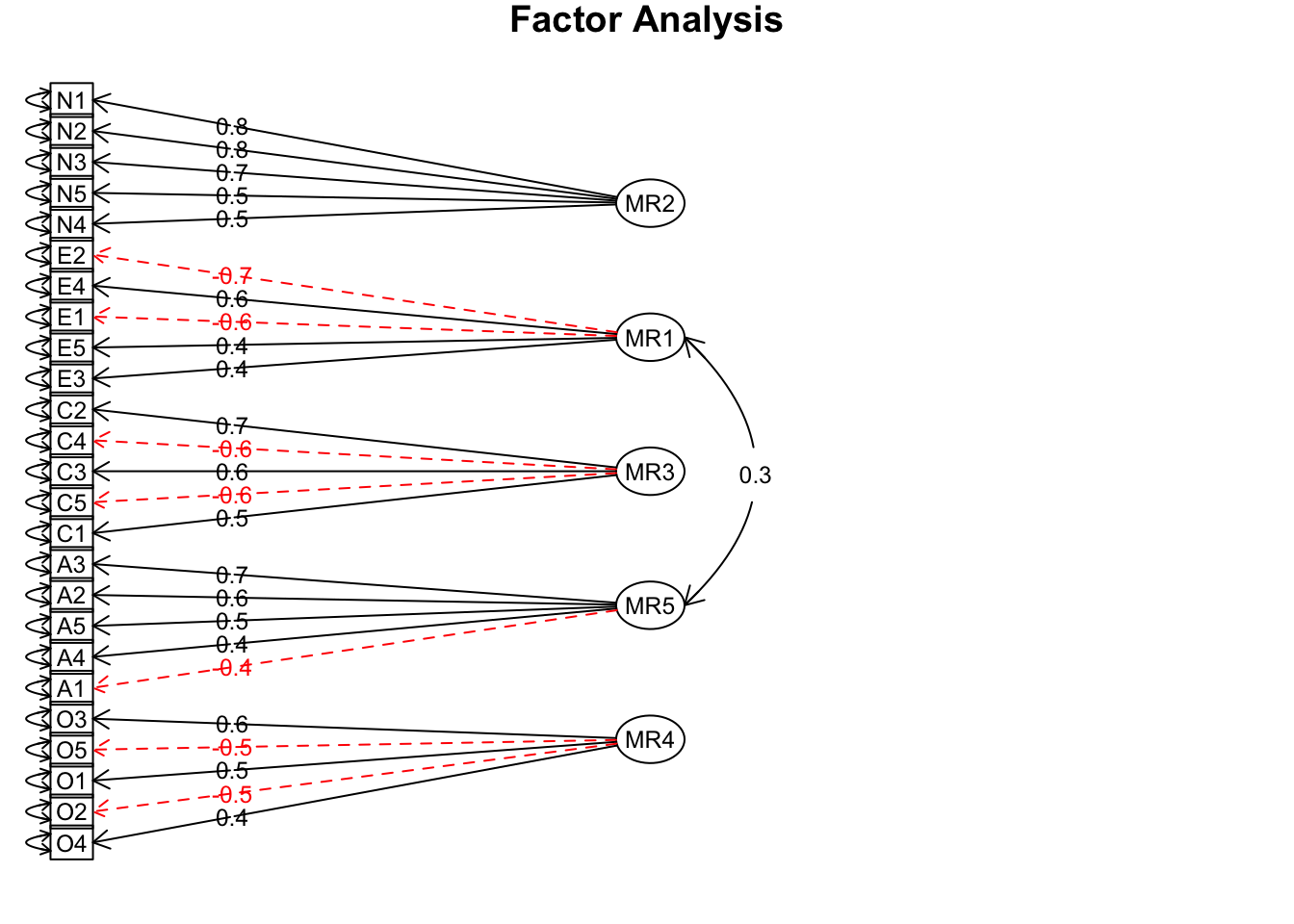
Interpretation
The factor diagram gives you a big picture sense of the solution: there are 5 factors, and the items vary in how much they load (correlate) with each factor. The output is a little harder to parse, but notice that items also correlate with other factors. Factors also correlate with other factors. You also get some model fit indices, which give you a sense of how much the model implied correlation matrix deviates from the original matrix (like residuals in regression). For more information about the output, see
help(fa).
Compare correlations among factors extracted from each model
Refit models to make later code easier to read (i.e., so you don’t have to read code for one function nested inside another function)
# fit principal componenets analysis
principal.fit1 <- principal(bfi25, nfactors = 5, rotate = "varimax")

# fit factor analysis
fa.fit1 <- fa(bfi25, nfactors = 5, rotate = "oblimin", fm = "minres")
Are the factors and components congruent?
help(factor.congruence)
“Given two sets of factor loadings, report their degree of congruence (vector cosine). Although first reported by Burt (1948), this is frequently known as the Tucker index of factor congruence.”
factor.congruence(list(principal.fit1, fa.fit1)) %>%
  as.data.frame() %>%
  mutate(factor1 = rownames(.)) %>%
  gather(key = factor2, value = r, -factor1) %>%
  ggplot(mapping = aes(x = factor1, y = factor2, fill = r, label = r)) +
  geom_tile() +
  geom_text() +
  scale_fill_gradient2()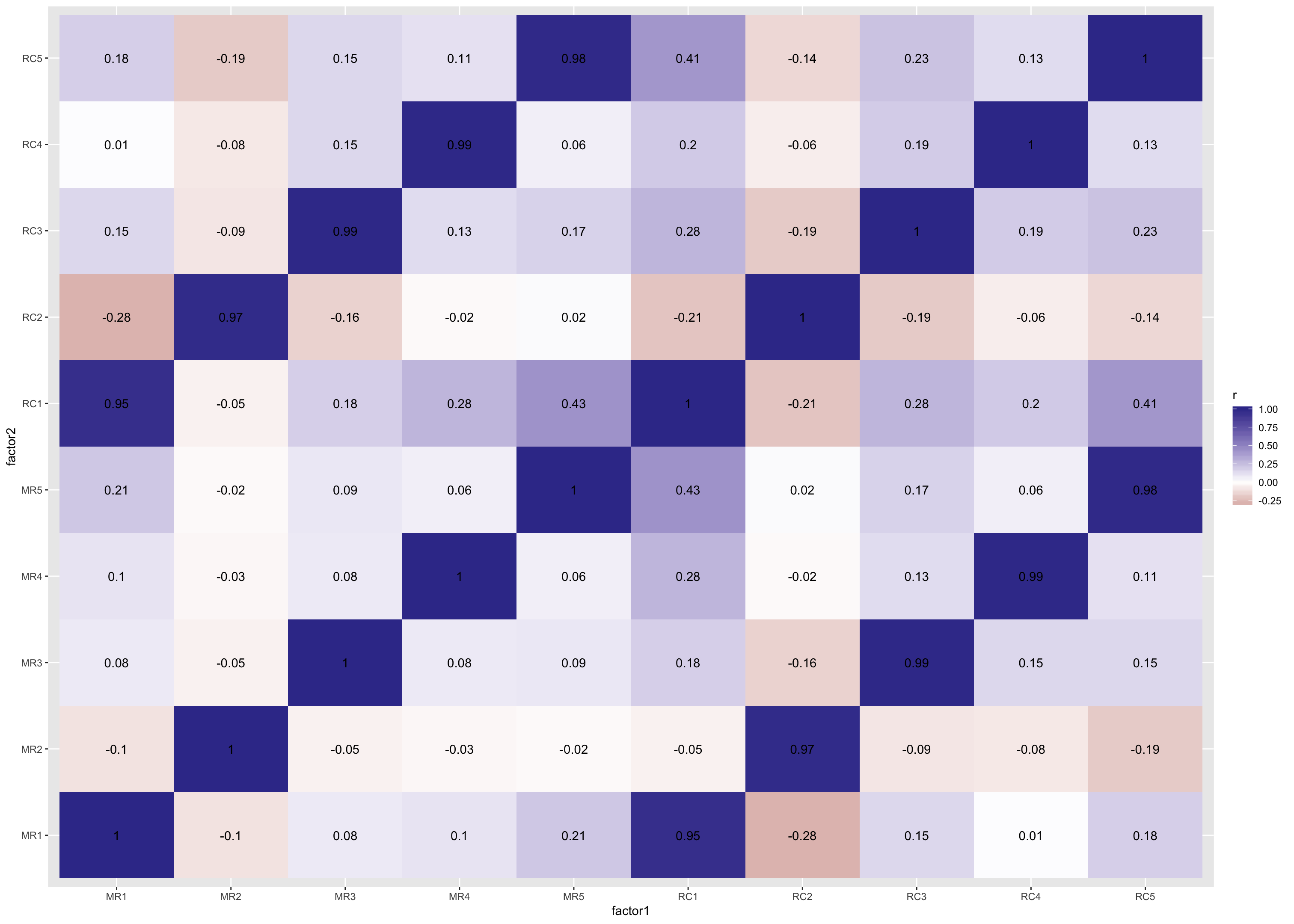
Interpretation
MR variables refer to factors from the common factor model, and RC variable refer to components from the components model. Darker blue tiles suggest two factors are more congruent, and whiter and darker red tiles suggest two “factors”1 are less congruent. These give you a sense of how different the loadings are depending on the model you use. In this case, we used one model that assumes all variance is common and the factors are uncorrelated (Component Analysis) and another model that assumes some variance is common but some is also special or due to error, and factors are correlated (Common Factor Analysis).
Full circle: Use the Non-Metric Multidimensional Scaling procedure on Big Five Inventory items
Save the correlation matrix and convert it to distance
help(corFiml)
“In the presence of missing data, Full Information Maximum Likelihood (FIML) is an alternative to simply using the pairwise correlations. The implementation in the lavaan package for structural equation modeling has been adapted for the simpler case of just finding the correlations or covariances.”
# save correlation matrix
r <- corFiml(bfi25)

# convert to distance matrix
bfi.d <- sqrt(2 * (1 - r))
Kruskal’s Non-metric Multidimensional Scaling
2-dimensions, because 5 dimensions would be bonkers
help(isoMDS)
“This chooses a k-dimensional (default k = 2) configuration to minimize the stress, the square root of the ratio of the sum of squared differences between the input distances and those of the configuration to the sum of configuration distances squared. However, the input distances are allowed a monotonic transformation.”
# give it distance values and number of dimensions
# also ask for the function to output eigenvalues
isoMDS.fit1 <- isoMDS(bfi.d, k = 2, maxit = 100)
## initial value 20.324535
## iter 5 value 14.753512
## iter 10 value 14.467916
## iter 10 value 14.460913
## iter 10 value 14.459080
## final value 14.459080
## convergedGenerate Shepard plot
This helps diagnose whether a monotonic relationship makes sense (i.e., when x goes up, y goes up)
Here’s an ideal monotonic relationship
As x goes up, y always goes up
tibble(x = 1:5, y = x + c(1, 2, 5, 8, 20)) %>%
  ggplot(mapping = aes(x = x, y = y)) +
  geom_point() +
  geom_line()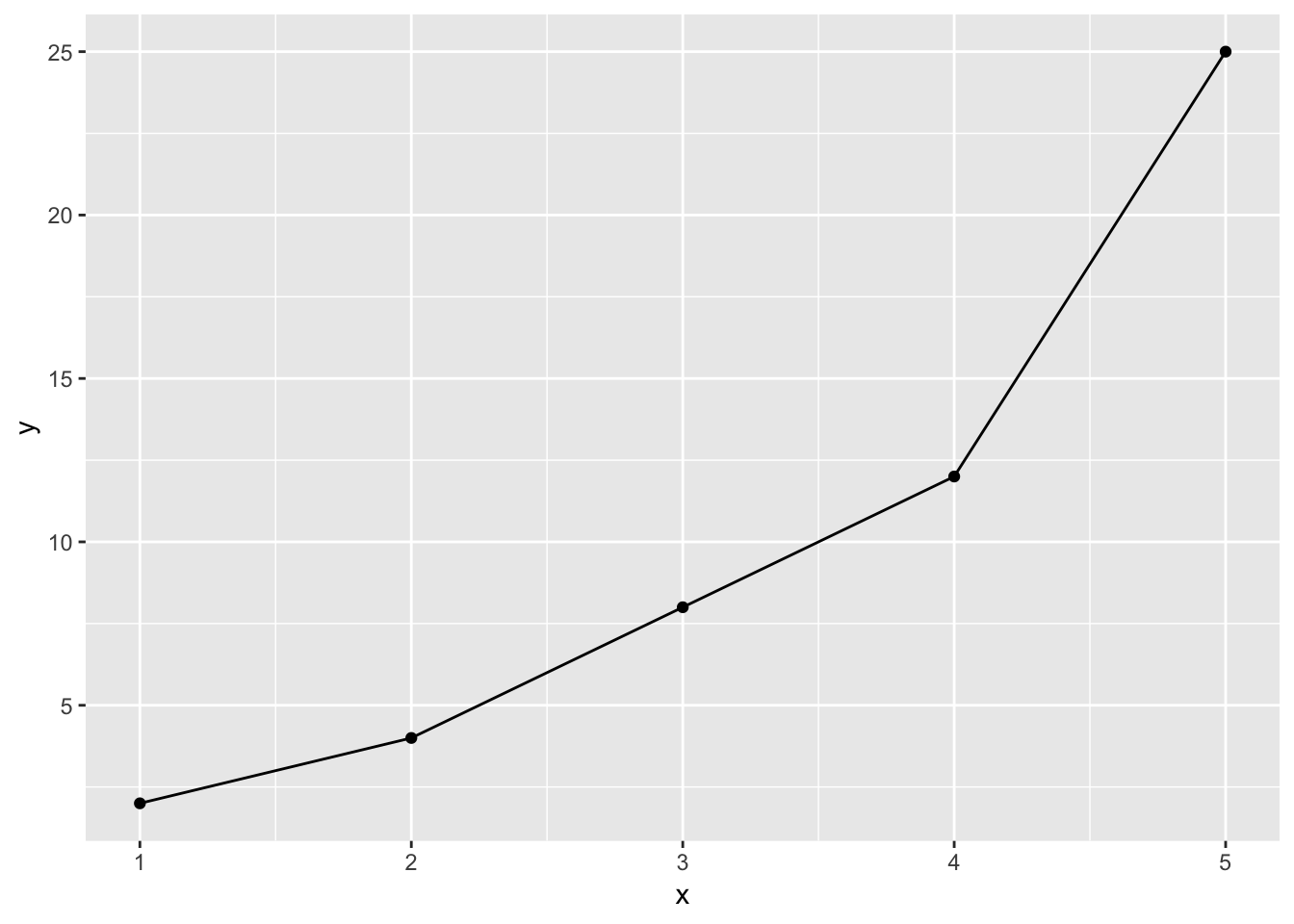
Compare to the non-metric Multidimensional Scaling Solution
# shepard
Shepard.fit1 <- Shepard(as.dist(bfi.d), isoMDS.fit1$points)

# save the values from the 2 dimensions (x and y) and the predicted/fitted values (yf)
shepard.data1 <- tibble(x = Shepard.fit1$x, y = Shepard.fit1$y, fit = Shepard.fit1$yf)

# plot
shepard.data1 %>%
  ggplot(mapping = aes(x = x, y = y)) +
  geom_point(alpha = 0.5) +
  geom_line(mapping = aes(x = x, y = fit))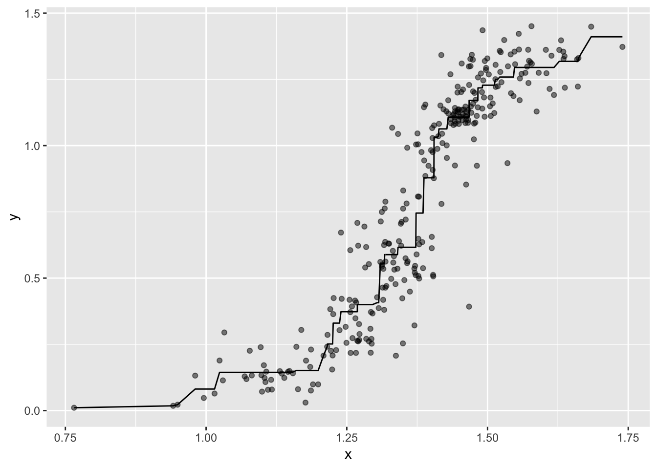
Interpretation
In these data, sometimes when x values went up, y values went down. To maintain this ordinal relationship, the algorithm “averages” the values so that the fitted line never goes down (i.e., it never reverses the up-and-then-up-again relationship). Compare the fitted line to the example of an ideal monotonic relationship above. Notice the plateaus. Some plateaus are fine, but those long plateaus at the start of the fitted line aren’t ideal. I’m going to move on with the rest of the demonstration, but in real-life data analysis you might want to investigate these data further (e.g., look for subsets of items an apply non-metric MDS to each, use metric MDS instead).
Store points from the fitted configuration/solution in a tibble data.frame
- The first and second dimension are stored as columns in the
pointsobject from theisoMDSfunction
- I use the ifelse and str_detect functions to create a trait variable that identifies the trait the item is supposed to “tap into.”
isoMDS.data1 <- tibble(item = rownames(isoMDS.fit1$points),
                       dimension1 = isoMDS.fit1$points[, 1],
                       dimension2 = isoMDS.fit1$points[, 2],
                       trait = ifelse(str_detect(item, pattern = "A"), "Agreeableness",
                               ifelse(str_detect(item, pattern = "C"), "Conscientiousness",
                               ifelse(str_detect(item, pattern = "E"), "Extraversion",
                               ifelse(str_detect(item, pattern = "N"), "Emotional Stability",
                               ifelse(str_detect(item, pattern = "O"), "Openness", NA))))))
Plot the (imperfect) 2-dimension solution
isoMDS.data1 %>%
  ggplot(mapping = aes(x = dimension1, y = dimension2, label = item, color = trait)) +
  geom_point() +
  geom_text(nudge_x = 0.025) +
  theme(legend.position = "top")
Interpretation
To be rigorous, I used a non-metric version of Multidimensional Scaling that uses a “monotonic” function (i.e., ordinal, non-linear) to find a solution. I only asked for 2 dimensions, so the solution doesn’t quite capture all the meaningful information contained in these 25 questions. However, you can still tell that items that tap into a given trait tend to “land” in a similar space on the plot as their “friends” (i.e., N items land next to other N items). Some items don’t land among their trait friends because they were negatively worded (no N items were negatively worded, so they all landed together). For example, had I negatively scored item C4 (“Do things in a half-way manner.”) and item C5 (“Waste my time.”), those items would likely have landed with item C1 (“Am exacting in my work.”), item C2 (“Continue until everything is perfect.”), and item C3 (“Do things according to a plan.”). So, given the information it had to work with, the Non-Metric Multidimensional Scaling procedure did a pretty good job!
Footnotes
- Although it many cases it’s useful to distinguish between factors and components (I do in this post), the information you need to interpret differences in solutions boils down to differences among models, not terms. Here’s a case where it’s confusing to refer to factors and components because it makes it seems like the congruence test is comparing apples to oranges; but it’s comparing “factor” (or “component”) solutions from two different models.
Resources
- Gonzalez, R. (February, 2016). Lecture Notes #10: MDS & Tree Structures. Retrieved from http://www-personal.umich.edu/~gonzo/coursenotes/file10.pdf on February 17, 2019.
- Revelle, W. (n.d.). An introduction to psychometric theory with applications in R. Retreived from http://www.personality-project.org/r/book/ on February 17, 2019.
- A practical introduction to factor analysis: exploratory factor analysis. UCLA: Statistical Consulting Group. Retreived from https://stats.idre.ucla.edu/spss/seminars/introduction-to-factor-analysis/a-practical-introduction-to-factor-analysis/ on February 17, 2019.
General word of caution
Above, I listed resources prepared by experts on these and related topics. Although I generally do my best to write accurate posts, don’t assume my posts are 100% accurate or that they apply to your data or research questions. Trust statistics and methodology experts, not blog posts.
Nicholas M. Michalak
Data Scientist | Ph.D. Social Psychology
I study how both modern and evolutionarily-relevant threats affect how people perceive themselves and others.